
Note
Go to the end to download the full example code or to run this example in your browser via Binder.
Scale pose tracks to real-world units#
Convert pixel coordinates to physical units using a known reference distance.
Acknowledgements
This example was originally contributed by Holly Morley—a PhD student at the Sainsbury Wellcome Centre studying sensory-guided predictive movements in mice—and uses data she collected for her PhD project.
Imports#
import numpy as np
from matplotlib import pyplot as plt
from scipy.signal import find_peaks

from movement import sample_data
from movement.filtering import (
    filter_by_confidence,
    interpolate_over_time,
    rolling_filter,
)
from movement.kinematics import compute_pairwise_distances
from movement.transforms import scale
Load sample dataset#
In this example, we will use the DLC_single-mouse_DBTravelator_2D
sample dataset, which contains DeepLabCut predictions of a single
mouse running across a dual-belt travelator, where the second belt
runs faster than the first.
The back wall of the travelator has a visible 1 cm grid, which we can use as a scaling reference to convert pixel coordinates into real-world units.
ds = sample_data.fetch_dataset(
    "DLC_single-mouse_DBTravelator_2D.predictions.h5", with_video=True
)
print(ds)
<xarray.Dataset> Size: 508kB
Dimensions:     (time: 418, space: 2, keypoint: 50, individual: 1)
Coordinates:
  * time        (time) float64 3kB 0.0 0.004049 0.008097 ... 1.68 1.684 1.688
  * space       (space) <U1 8B 'x' 'y'
  * keypoint    (keypoint) <U15 3kB 'StartPlatL' 'StepL' ... 'HindpawKneeL'
  * individual  (individual) <U12 48B 'individual_0'
Data variables:
    position    (time, space, keypoint, individual) float64 334kB 70.12 ... 1...
    confidence  (time, keypoint, individual) float64 167kB 1.0 1.0 ... 0.005941
Attributes:
    source_software:  DeepLabCut
    ds_type:          poses
    fps:              247.0
    time_unit:        seconds
    source_file:      /home/runner/.movement/data/poses/DLC_single-mouse_DBTr...
    frame_path:       /home/runner/.movement/data/frames/single-mouse_DBTrave...
    video_path:       /home/runner/.movement/data/videos/single-mouse_DBTrave...
We can see the DeepLabCut dataset contains positions and confidence scores for 50 keypoints tracked on a single mouse, recorded at 247 fps over approximately 1.7 seconds.
Prepare the dataset#
Before scaling, let’s inspect the tracked keypoints and clean up the data.
We can see that out of the 50 tracked keypoints, the majority track positions along the mouse’s body (head, back, tail, and limbs).
print(ds.keypoint.values)
['StartPlatL' 'StepL' 'StartPlatR' 'StepR' 'Door' 'TransitionL'
 'TransitionR' 'Nose' 'EarL' 'EarR' 'Back1' 'Back2' 'Back3' 'Back4'
 'Back5' 'Back6' 'Back7' 'Back8' 'Back9' 'Back10' 'Back11' 'Back12'
 'Tail1' 'Tail2' 'Tail3' 'Tail4' 'Tail5' 'Tail6' 'Tail7' 'Tail8' 'Tail9'
 'Tail10' 'Tail11' 'Tail12' 'ForepawToeR' 'ForepawKnuckleR'
 'ForepawAnkleR' 'ForepawKneeR' 'ForepawToeL' 'ForepawKnuckleL'
 'ForepawAnkleL' 'ForepawKneeL' 'HindpawToeR' 'HindpawKnuckleR'
 'HindpawAnkleR' 'HindpawKneeR' 'HindpawToeL' 'HindpawKnuckleL'
 'HindpawAnkleL' 'HindpawKneeL']
However, there are also a number of keypoints which track physical landmarks on the apparatus rather than the mouse itself. We don’t need these so we can filter them out of the dataset.
landmark_keypoints = [
    "Door",
    "StartPlatL",
    "StartPlatR",
    "StepL",
    "StepR",
    "TransitionL",
    "TransitionR",
]

# Select all keypoints excluding the landmarks, and the single individual.
ds_mouse = ds.sel(
    keypoint=~ds.keypoint.isin(landmark_keypoints),
    individual="individual_0",
)

print(ds_mouse)
print("----------------------------------")
print(f"Keypoints:\n{ds_mouse.keypoint.values}")
<xarray.Dataset> Size: 437kB
Dimensions:     (time: 418, space: 2, keypoint: 43)
Coordinates:
  * time        (time) float64 3kB 0.0 0.004049 0.008097 ... 1.68 1.684 1.688
  * space       (space) <U1 8B 'x' 'y'
  * keypoint    (keypoint) <U15 3kB 'Nose' 'EarL' ... 'HindpawKneeL'
    individual  <U12 48B 'individual_0'
Data variables:
    position    (time, space, keypoint) float64 288kB 55.6 47.47 ... 201.7 170.1
    confidence  (time, keypoint) float64 144kB 0.02365 0.01434 ... 0.005941
Attributes:
    source_software:  DeepLabCut
    ds_type:          poses
    fps:              247.0
    time_unit:        seconds
    source_file:      /home/runner/.movement/data/poses/DLC_single-mouse_DBTr...
    frame_path:       /home/runner/.movement/data/frames/single-mouse_DBTrave...
    video_path:       /home/runner/.movement/data/videos/single-mouse_DBTrave...
----------------------------------
Keypoints:
['Nose' 'EarL' 'EarR' 'Back1' 'Back2' 'Back3' 'Back4' 'Back5' 'Back6'
 'Back7' 'Back8' 'Back9' 'Back10' 'Back11' 'Back12' 'Tail1' 'Tail2'
 'Tail3' 'Tail4' 'Tail5' 'Tail6' 'Tail7' 'Tail8' 'Tail9' 'Tail10' 'Tail11'
 'Tail12' 'ForepawToeR' 'ForepawKnuckleR' 'ForepawAnkleR' 'ForepawKneeR'
 'ForepawToeL' 'ForepawKnuckleL' 'ForepawAnkleL' 'ForepawKneeL'
 'HindpawToeR' 'HindpawKnuckleR' 'HindpawAnkleR' 'HindpawKneeR'
 'HindpawToeL' 'HindpawKnuckleL' 'HindpawAnkleL' 'HindpawKneeL']
Next we remove low-confidence predictions, interpolate over gaps, and apply a rolling median filter to suppress any remaining tracking outliers.
ds_mouse["position"] = filter_by_confidence(
    ds_mouse.position,
    ds_mouse.confidence,
    threshold=0.9,
)
ds_mouse["position"] = interpolate_over_time(ds_mouse.position, max_gap=40)
ds_mouse["position"] = rolling_filter(
    ds_mouse.position,
    window=6,
    min_periods=2,
    statistic="median",
)
Visualise the skeleton in pixels#
To see what the pose data looks like before scaling, we define a helper function that draws the mouse skeleton in a single frame.
def plot_skeleton(position_data, skeleton, frame, ax, s=3):
    """Plot the mouse skeleton for a single frame.

    Parameters
    ----------
    position_data : xarray.DataArray
        Position data with dimensions ``time``, ``keypoint``, and ``space``.
    skeleton : list of tuple
        List of (joint_1, joint_2) pairs defining skeletal connections,
        where each element is a keypoint name present in ``position_data``.
    frame : int
        Index of the time frame to plot.
    ax : matplotlib.axes.Axes
        Axes on which to draw.
    s : float, optional
        Marker size for keypoint scatter points. Default is 3.

    """
    pos_frame = position_data.squeeze().isel(time=frame)

    # Draw skeleton connections
    for joint_1, joint_2 in skeleton:
        x1, y1 = pos_frame.sel(keypoint=joint_1)
        x2, y2 = pos_frame.sel(keypoint=joint_2)
        ax.plot([x1, x2], [y1, y2], color="b", linewidth=1.5)

    # Draw keypoints
    for bodypart in pos_frame.keypoint:
        x, y = pos_frame.sel(keypoint=bodypart)
        ax.scatter(x, y, c="g", s=s)
We define the connections between keypoints that form the mouse skeleton, then plot it for a single frame using the above function.
skeleton = [
    ("Nose", "Back1"),
    ("EarL", "Back1"),
    ("EarR", "Back1"),
    ("Back1", "Back2"),
    ("Back2", "Back3"),
    ("Back3", "Back4"),
    ("Back4", "Back5"),
    ("Back5", "Back6"),
    ("Back6", "Back7"),
    ("Back7", "Back8"),
    ("Back8", "Back9"),
    ("Back9", "Back10"),
    ("Back10", "Back11"),
    ("Back11", "Back12"),
    ("Back12", "Tail1"),
    ("Tail1", "Tail2"),
    ("Tail2", "Tail3"),
    ("Tail3", "Tail4"),
    ("Tail4", "Tail5"),
    ("Tail5", "Tail6"),
    ("Tail6", "Tail7"),
    ("Tail7", "Tail8"),
    ("Tail8", "Tail9"),
    ("Tail9", "Tail10"),
    ("Tail10", "Tail11"),
    ("Tail11", "Tail12"),
    ("Back3", "ForepawKneeL"),
    ("Back3", "ForepawKneeR"),
    ("Back9", "HindpawKneeL"),
    ("Back9", "HindpawKneeR"),
    ("ForepawKneeL", "ForepawAnkleL"),
    ("ForepawKneeR", "ForepawAnkleR"),
    ("HindpawKneeL", "HindpawAnkleL"),
    ("HindpawKneeR", "HindpawAnkleR"),
    ("ForepawAnkleL", "ForepawKnuckleL"),
    ("ForepawAnkleR", "ForepawKnuckleR"),
    ("HindpawAnkleL", "HindpawKnuckleL"),
    ("HindpawAnkleR", "HindpawKnuckleR"),
    ("ForepawKnuckleL", "ForepawToeL"),
    ("ForepawKnuckleR", "ForepawToeR"),
    ("HindpawKnuckleL", "HindpawToeL"),
    ("HindpawKnuckleR", "HindpawToeR"),
]

example_frame = 275

fig, ax = plt.subplots(figsize=(8, 3))
plot_skeleton(ds_mouse.position, skeleton, frame=example_frame, ax=ax, s=10)

ax.invert_yaxis()  # image coordinates have y increasing downward
ax.set_xlabel("x (pixels)")
ax.set_ylabel("y (pixels)")
ax.set_aspect("equal")
plt.show()
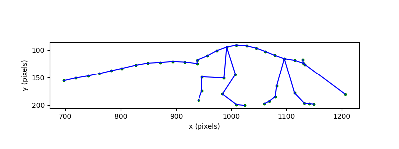
The skeleton gives us the shape of the mouse’s body, but the coordinate
system is in pixels. To interpret sizes and distances in real-world units,
we need to convert to physical units. We can do this by measuring a known
distance in the video using the napari GUI and then applying
movement.transforms.scale() to convert from pixels to centimetres.
Measure a known distance from video footage#
Attention
The following steps require running this example locally (not on
Binder), with napari installed. If you haven’t already, install
movement with the optional napari dependencies by following the
installation instructions.
First, open the video file (or a single video frame) in napari by running
the following code in a Jupyter notebook:
import napari
viewer = napari.Viewer()
viewer.open(ds_mouse.video_path)  # can also use ds_mouse.frame_path
Note
Alternatively, you can type napari in a terminal, wait for the
viewer to open, and drag-and-drop the video/frame file into the viewer.
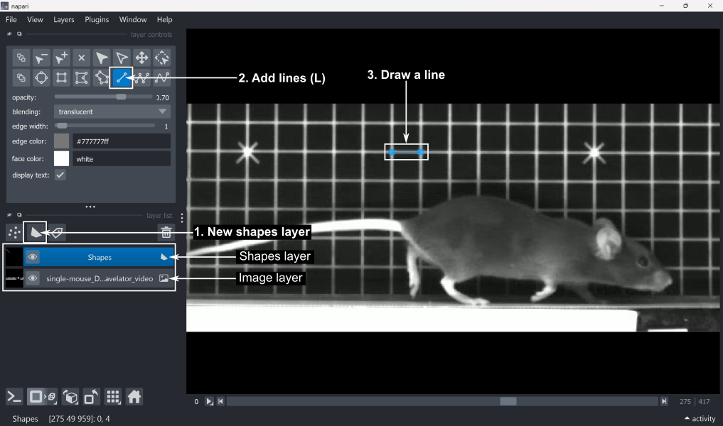
Next, measure a known distance in the napari viewer:
Add a new shapes layer by clicking ‘New shapes layer’ in the layer list.
Select the ‘Add lines’ tool (shortcut: L) from the layer controls.
Draw a line across a feature of known length. In this case, the grid squares are 1x1 cm, so we can draw a line along one side of a grid square.
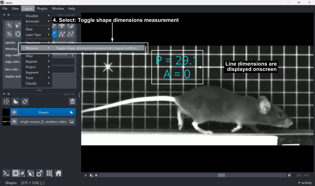
4. To read the line length in pixels, go to Layers → Measure → Toggle shape dimensions measurement (napari builtins). This displays P (perimeter) and A (area). In the case of a single line, the perimeter value corresponds to the line length in pixels, and the area will always be 0.
Close the
napariviewer.
We can then retrieve the measured distance and line coordinates from the shapes layer.
shapes_layer = viewer.layers["Shapes"]
measurements_px = shapes_layer.features
shape_coords = shapes_layer.data

print(f"Measurements:\n{measurements_px}\n")
print(f"Coordinates:\n{shape_coords}")

# Extract the line length in pixels from the perimeter (P) column
distance_px = measurements_px["_perimeter"].values.squeeze()
Measurements:
   _perimeter  _area
0   29.063293    0.0

Coordinates:
[array([[275.      ,  48.455124, 930.55444 ],
       [275.      ,  48.452595, 959.61774 ]], dtype=float32)]
Transform poses to real units#
We now transform the pose coordinates to real-world units in two steps: scaling from pixels to centimetres, and flipping the y-axis so that positive y corresponds to upward in real-world space (image coordinates have the y-axis pointing downward).
First, we calculate the scaling factor. The measured line spans one grid square, which we know to be 1 cm. Dividing this known length by the distance in pixels gives us the scaling factor.
scaling_factor = 1 / distance_px
print(f"Scaling factor: {scaling_factor:.6f} cm/pixel")
Scaling factor: 0.034408 cm/pixel
Note
This scaling factor assumes a constant relationship between pixels and real-world units across the entire image, based on a single reference measurement taken at the far side of the belt. In practice, several factors can violate this assumption. For example, in 2D imaging, perspective effects mean that the apparent size of objects varies with their distance from the camera. Distances measured in the plane of the reference grid will therefore be close to accurate, but can deviate as the mouse moves away from this plane. Calibrated multi-camera setups avoid these assumptions by mapping image coordinates directly to real-world 3D space.
Let’s inspect the position values before scaling.
# Select a frame range in which the mouse is visible
sample_range = np.arange(300, 301)
print(ds_mouse.position.isel(time=sample_range).values)
[[[1398.2734375  1321.61193848 1330.91986084 1324.80633545 1306.98193359
   1288.26031494 1270.04632568 1252.95697021 1235.85125732 1217.36029053
   1199.72625732 1181.1987915  1163.58392334 1146.29034424 1126.3626709
   1126.17126465 1103.95812988 1081.17657471 1057.53509521 1035.8026123
   1012.95870972  988.29507446  968.99377441  946.29476929  925.46606445
    903.1199646   882.91726685 1299.08605957 1289.45465088 1281.8973999
   1283.18951416 1340.15515137 1337.95861816 1327.96911621 1313.1293335
   1192.83721924 1185.10662842 1160.95397949 1195.93652344 1151.7109375
   1136.6963501  1134.84191895 1168.97979736]
  [ 179.98707581  114.40616608  126.98419189  124.15420151  118.58591843
    116.37707901  113.20304489  108.78902054  104.51488113  100.12917328
     97.42570114   98.87822342  104.46193314  111.52003479  118.15843201
    124.30410385  119.9714241   116.60536957  115.4688797   114.47219467
    115.20085907  118.57863998  118.48215866  121.45074081  121.86370087
    123.55347824  125.70636749  200.3639679   199.53270721  196.58586884
    173.59635162  192.48999023  185.47390747  180.66627502  170.02613068
    192.91704559  179.59600067  163.21473694  142.73191833  200.17955017
    194.60357666  166.07353973  161.26473236]]]
Now we apply movement.transforms.scale() to convert from pixels to
centimetres. We can assign our space unit ‘cm’ here, to be stored as an
attribute in xarray.DataArray.attrs['space_unit'].
ds_mouse["position"] = scale(
    ds_mouse["position"], factor=scaling_factor, space_unit="cm"
)
Now we inspect our sample of values again. We can see the values have been adjusted.
print(ds_mouse.position.isel(time=sample_range).values)
[[[48.11132164 45.4735786  45.79384245 45.58349033 44.97019431
   44.32602716 43.69932635 43.11132156 42.52275395 41.88652299
   41.27977712 40.64229031 40.03620386 39.44117221 38.75550754
   38.74892169 37.98461963 37.20075955 36.38731149 35.63954753
   34.85354222 34.00492417 33.34081153 32.55979181 31.84312474
   31.07424766 30.37912004 44.69851574 44.36712147 44.10709412
   44.15155276 46.11160722 46.03602965 45.69231423 45.18171198
   41.04274141 40.77674985 39.94571364 41.14938123 39.62768216
   39.11106529 39.04725865 40.22186327]
  [ 6.1929347   3.93644884  4.36922932  4.27185596  4.08026435
    4.00426335  3.89505225  3.74317599  3.59611284  3.44521088
    3.35219072  3.40216862  3.59429102  3.83714381  4.06555554
    4.27701375  4.12793637  4.0121183   3.97301433  3.93872073
    3.96379237  4.08001392  4.07669422  4.1788362   4.19304519
    4.25118648  4.32526237  6.89405595  6.86545421  6.76406038
    5.97304482  6.62313077  6.38172376  6.21630436  5.85020186
    6.63782475  6.17947872  5.61583771  4.91107179  6.88771056
    6.69585434  5.71420244  5.54874261]]]
The scaled data array’s attributes now contain the space_unit and a
log entry recording the operation and its parameters, alongside the
operations applied in earlier steps.
Unit:
cm

Log:
[
  {
    "operation": "filter_by_confidence",
    "datetime": "2026-06-08 16:33:26.770105",
    "confidence": "<xarray.DataArray 'confidence' (time: 418, keypoint: 43)> Size: 144kB\n0.02365 0.01434 0.01821 0.02692 0.05129 ... 0.004628 0.007376 0.003921 0.005941\nCoordinates:\n  * time        (time) float64 3kB 0.0 0.004049 0.008097 ... 1.68 1.684 1.688\n  * keypoint    (keypoint) <U15 3kB 'Nose' 'EarL' ... 'HindpawKneeL'\n    individual  <U12 48B 'individual_0'",
    "threshold": "0.9",
    "print_report": "False"
  },
  {
    "operation": "interpolate_over_time",
    "datetime": "2026-06-08 16:33:26.782927",
    "method": "'linear'",
    "max_gap": "40",
    "print_report": "False"
  },
  {
    "operation": "rolling_filter",
    "datetime": "2026-06-08 16:33:26.785616",
    "window": "6",
    "statistic": "'median'",
    "min_periods": "2",
    "print_report": "False"
  },
  {
    "operation": "scale",
    "datetime": "2026-06-08 16:33:27.026768",
    "factor": "np.float64(0.03440766330229682)",
    "space_unit": "'cm'"
  }
]
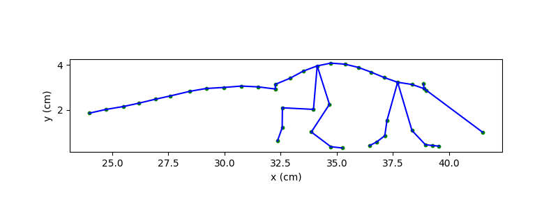
Next, we flip the y-axis by subtracting each y value from the maximum y value in the dataset. Note that the zero point in y is anchored to the lowest y position of the mouse in this recording, which approximates the belt surface.
We can now re-plot the same skeleton, this time in centimetres and with the y-axis pointing upward.
fig, ax = plt.subplots(figsize=(8, 3))
plot_skeleton(ds_mouse.position, skeleton, frame=example_frame, ax=ax, s=10)

ax.set_xlabel("x (cm)")
ax.set_ylabel("y (cm)")
ax.set_aspect("equal")
plt.show()
Working with real-world distances#
With the data now in centimetres, we can measure the mouse directly. Let’s
first compute its approximate body length and height in example_frame.
frame_x = ds_mouse.position.sel(space="x").isel(time=example_frame)
frame_y = ds_mouse.position.sel(space="y").isel(time=example_frame)

mouse_length = frame_x.sel(keypoint="Nose") - frame_x.sel(keypoint="Tail12")
mouse_height = frame_y.max() - frame_y.min()

print(f"Mouse length: {mouse_length.values:.1f} cm")
print(f"Mouse height: {mouse_height.values:.1f} cm")
Mouse length: 17.5 cm
Mouse height: 3.8 cm
Beyond simple static measurements, real-world units also make aspects of movement, such as gait-related distances interpretable. Let’s visualise the paw trajectories in x and y over time.
# Select the toe keypoints for all four limbs
toe_keypoint_names = [
    "ForepawToeR",
    "ForepawToeL",
    "HindpawToeR",
    "HindpawToeL",
]

# Construct a new data array with only the toe keypoints
ds_limbs = ds_mouse.position.sel(keypoint=toe_keypoint_names)

ds_limbs.plot.line(
    x="time",
    hue="keypoint",
    row="space",
    size=2.5,
    aspect=2,
    sharey=False,
)
axs = plt.gcf().axes
axs[0].set_ylabel("x (cm)")
axs[1].set_xlabel("Time (s)")
axs[1].set_ylabel("y (cm)")
plt.show()
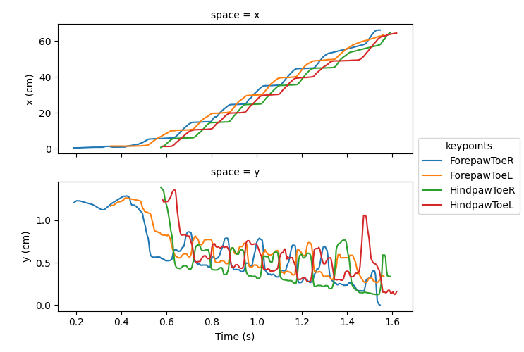
Here we see the mouse traverses approximately 60 cm across the travelator, and step heights typically remain below around 0.5 cm.
These trajectories give us a broad sense of limb movement, but we can go
further and quantify dynamics between limbs, such as the inter-limb
distances in real-world units using
movement.kinematics.compute_pairwise_distances(). Here, we again use
the toe keypoints to compare the anterior-posterior separation of the fore-
and hindpaw pairs.
forepaw_dist = compute_pairwise_distances(
    ds_mouse.position,
    dim="keypoint",
    pairs={"ForepawToeL": "ForepawToeR"},
)
hindpaw_dist = compute_pairwise_distances(
    ds_mouse.position,
    dim="keypoint",
    pairs={"HindpawToeL": "HindpawToeR"},
)
We plot these inter-limb distances for the fore- and hindpaws against the mean x-position of the body as the mouse traverses the travelator. Since we know the first belt is 47 cm long, we can also easily plot the transition point at which the mouse moves onto the faster second belt.
belt_transition = 47  # cm

# Compute a proxy for body centre in x
avg_body_x = ds_mouse.position.sel(space="x").mean(dim="keypoint")

fig, ax = plt.subplots()
ax.plot(avg_body_x, forepaw_dist, color="tab:blue", label="Forepaws")
ax.plot(avg_body_x, hindpaw_dist, color="tab:orange", label="Hindpaws")
ax.axvline(belt_transition, color="k", linestyle="--", label="Belt transition")

ax.set_xlabel("x (cm)")
ax.set_ylabel("Inter-limb distance (cm)")
plt.legend()
plt.show()
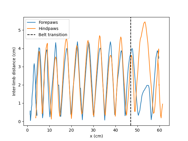
The forepaw and hindpaw inter-limb distances oscillate largely in synchrony, consistent with a trotting gait, with peak separations of approximately 4 cm for the majority of strides.
However, after the mouse’s body centre passes the belt transition, the forepaw inter-limb distance drops noticeably whilst the hindpaw distance increases. This likely reflects the mouse accommodating the speed difference between belts - the forepaws shorten their stride to avoid over-reaching, while the hindpaws widen to keep the rear of the body from trailing behind.
We can quantify these observations by comparing peak inter-limb distances across all strides with those during only the transitioning stride.
First, let’s compute the mean peak inter-limb distance across all strides.
# Find maximum interlimb distances in each stride by locating the peaks.
forepaw_peaks, _ = find_peaks(forepaw_dist.values.squeeze(), prominence=0.2)
hindpaw_peaks, _ = find_peaks(hindpaw_dist.values.squeeze(), prominence=0.2)

# Find inter-limb distances at these peak locations
forepaw_peak_vals = forepaw_dist.values.squeeze()[
    forepaw_peaks[2:]
]  # Exclude the first two peaks to match the available hindpaw strides
hindpaw_peak_vals = hindpaw_dist.values.squeeze()[hindpaw_peaks]

forepaw_mean = forepaw_peak_vals.mean()
hindpaw_mean = hindpaw_peak_vals.mean()

forepaw_std = forepaw_peak_vals.std()
hindpaw_std = hindpaw_peak_vals.std()

paw_diffs = hindpaw_peak_vals - forepaw_peak_vals
paw_diffs_mean = np.mean(paw_diffs)
paw_diffs_std = np.std(paw_diffs)

print(
    f"Mean peak inter-limb distance (forepaws): "
    f"{forepaw_mean:.2f} ± {forepaw_std:.2f} cm (± std)"
)
print(
    f"Mean peak inter-limb distance (hindpaws): "
    f"{hindpaw_mean:.2f} ± {hindpaw_std:.2f} cm (± std)"
)
print(
    f"Hindpaw - forepaw inter-limb difference: "
    f"{paw_diffs_mean:.2f} ± {paw_diffs_std:.2f} cm (± std)"
)
Mean peak inter-limb distance (forepaws): 3.92 ± 0.62 cm (± std)
Mean peak inter-limb distance (hindpaws): 4.23 ± 0.54 cm (± std)
Hindpaw - forepaw inter-limb difference: 0.31 ± 1.07 cm (± std)
Now let’s compare these average distances with the maximum inter-limb distances during the transitioning stride where the mouse steps onto the faster second belt (the second-to-last peak in each trace).
post_forepaw_dist = forepaw_dist.values.squeeze()[forepaw_peaks[-2]]
post_hindpaw_dist = hindpaw_dist.values.squeeze()[hindpaw_peaks[-2]]

print(
    f"Transitioning forepaw inter-limb distance:  {post_forepaw_dist:.2f} cm"
)
print(
    f"Transitioning hindpaw inter-limb distance:  {post_hindpaw_dist:.2f} cm"
)
print(
    f"Hindpaw–forepaw difference at transition:     "
    f"{post_hindpaw_dist - post_forepaw_dist:.2f} cm"
)
Transitioning forepaw inter-limb distance:  1.97 cm
Transitioning hindpaw inter-limb distance:  5.45 cm
Hindpaw–forepaw difference at transition:     3.48 cm
Here we can see that during typical locomotion, the fore- and hindpaw inter-limb distances are synchronised and closely matched, differing by only 0.31 cm on average. During the transitioning stride, however, this difference grows more than tenfold, reflecting the gait adjustments the mouse makes to accommodate the speed differential between belts.
Having the data in real-world units makes these quantitative comparisons possible.
Total running time of the script: (0 minutes 1.548 seconds)