Filtering and interpolation

Filter out points with low confidence scores and interpolate over missing values.

Imports

from movement import sample_data
from movement.filtering import filter_by_confidence, interpolate_over_time

Load a sample dataset

ds = sample_data.fetch_dataset("DLC_single-wasp.predictions.h5")
print(ds)

<xarray.Dataset> Size: 61kB
Dimensions:      (time: 1085, individuals: 1, keypoints: 2, space: 2)
Coordinates:
  * time         (time) float64 9kB 0.0 0.025 0.05 0.075 ... 27.05 27.07 27.1
  * individuals  (individuals) <U12 48B 'individual_0'
  * keypoints    (keypoints) <U7 56B 'head' 'stinger'
  * space        (space) <U1 8B 'x' 'y'
Data variables:
    position     (time, individuals, keypoints, space) float64 35kB 1.086e+03...
    confidence   (time, individuals, keypoints) float64 17kB 0.05305 ... 0.0
Attributes:
    fps:              40.0
    time_unit:        seconds
    source_software:  DeepLabCut
    source_file:      /home/runner/.movement/data/poses/DLC_single-wasp.predi...
    frame_path:       /home/runner/.movement/data/frames/single-wasp_frame-10...
    video_path:       None

We can see that this dataset contains the 2D pose tracks and confidence scores for a single wasp, generated with DeepLabCut. There are 2 keypoints: “head” and “stinger”.

Visualise the pose tracks

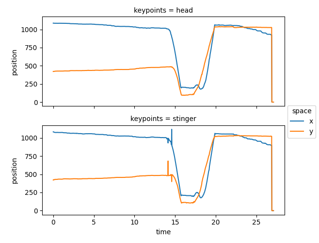
position = ds.position.sel(individuals="individual_0")
position.plot.line(x="time", row="keypoints", hue="space", aspect=2, size=2.5)

<xarray.plot.facetgrid.FacetGrid object at 0x7fca8518af10>

We can see that the pose tracks contain some implausible “jumps”, such as the big shift in the final second, and the “spikes” of the stinger near the 14th second. Perhaps we can get rid of those based on the model’s reported confidence scores?

Visualise confidence scores

The confidence scores are stored in the confidence data variable. Since the predicted poses in this example have been generated by DeepLabCut, the confidence scores should be likelihood values between 0 and 1. That said, confidence scores are not standardised across pose estimation frameworks, and their ranges can vary. Therefore, it’s always a good idea to inspect the actual confidence values in the data.

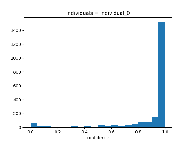
Let’s first look at a histogram of the confidence scores.

ds.confidence.plot.hist(bins=20)

(array([  61.,   13.,   16.,   10.,   10.,    8.,   21.,   11.,   14.,
         11.,   26.,   13.,   28.,   19.,   39.,   44.,   79.,   84.,
        149., 1514.]), array([0.        , 0.04999823, 0.09999646, 0.14999469, 0.19999292,
       0.24999115, 0.29998938, 0.34998761, 0.39998584, 0.44998407,
       0.4999823 , 0.54998053, 0.59997876, 0.64997699, 0.69997522,
       0.74997345, 0.79997168, 0.84996991, 0.89996814, 0.94996637,
       0.99996459]), <BarContainer object of 20 artists>)

Based on the above histogram, we can confirm that the confidence scores indeed range between 0 and 1, with most values closer to 1. Now let’s see how they evolve over time.

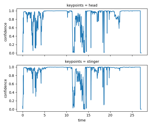
confidence = ds.confidence.sel(individuals="individual_0")
confidence.plot.line(x="time", row="keypoints", aspect=2, size=2.5)

<xarray.plot.facetgrid.FacetGrid object at 0x7fca852cd790>

Encouragingly, some of the drops in confidence scores do seem to correspond to the implausible jumps and spikes we had seen in the position. We can use that to our advantage.

Filter out points with low confidence

We can filter out points with confidence scores below a certain threshold. Here, we use threshold=0.6. Points in the position data variable with confidence scores below this threshold will be converted to NaN. The print_report argument, which is True by default, reports the number of NaN values in the dataset before and after the filtering operation.

ds_filtered = filter_by_confidence(ds, threshold=0.6, print_report=True)

Missing points (marked as NaN) in input dataset:
        Individual: individual_0
                head: 0/1085 (0.0%)
                stinger: 0/1085 (0.0%)

Missing points (marked as NaN) in filtered dataset:
        Individual: individual_0
                head: 121/1085 (11.2%)
                stinger: 93/1085 (8.6%)

We can see that the filtering operation has introduced NaN values in the position data variable. Let’s visualise the filtered data.

position_filtered = ds_filtered.position.sel(individuals="individual_0")
position_filtered.plot.line(
    x="time", row="keypoints", hue="space", aspect=2, size=2.5
)

<xarray.plot.facetgrid.FacetGrid object at 0x7fca874f2e50>

Here we can see that gaps have appeared in the pose tracks, some of which are over the implausible jumps and spikes we had seen earlier. Moreover, most gaps seem to be brief, lasting < 1 second.

Interpolate over missing values

We can interpolate over the gaps we’ve introduced in the pose tracks. Here we use the default linear interpolation method and max_gap=1, meaning that we will only interpolate over gaps of 1 second or shorter. Setting max_gap=None would interpolate over all gaps, regardless of their length, which should be used with caution as it can introduce spurious data. The print_report argument acts as described above.

ds_interpolated = interpolate_over_time(
    ds_filtered, method="linear", max_gap=1, print_report=True
)

Missing points (marked as NaN) in input dataset:
        Individual: individual_0
                head: 121/1085 (11.2%)
                stinger: 93/1085 (8.6%)

Missing points (marked as NaN) in interpolated dataset:
        Individual: individual_0
                head: 0/1085 (0.0%)
                stinger: 0/1085 (0.0%)

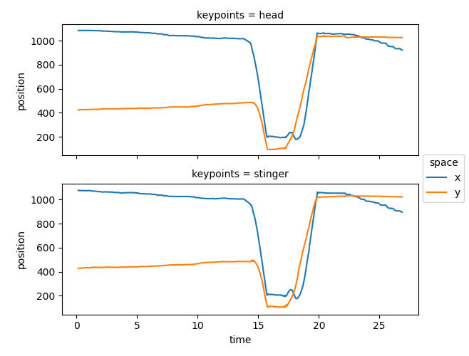
We see that all NaN values have disappeared, meaning that all gaps were indeed shorter than 1 second. Let’s visualise the interpolated pose tracks

position_interpolated = ds_interpolated.position.sel(
    individuals="individual_0"
)
position_interpolated.plot.line(
    x="time", row="keypoints", hue="space", aspect=2, size=2.5
)

<xarray.plot.facetgrid.FacetGrid object at 0x7fca87380150>

Log of processing steps

So, far we’ve processed the pose tracks first by filtering out points with low confidence scores, and then by interpolating over missing values. The order of these operations and the parameters with which they were performed are saved in the log attribute of the dataset. This is useful for keeping track of the processing steps that have been applied to the data.

for log_entry in ds_interpolated.log:
    print(log_entry)

{'operation': 'filter_by_confidence', 'datetime': '2024-05-15 08:49:30.096092', 'threshold': 0.6, 'print_report': True}
{'operation': 'interpolate_over_time', 'datetime': '2024-05-15 08:49:31.516639', 'method': 'linear', 'max_gap': 1, 'print_report': True}