Compute and visualise kinematics.

Compute displacement, velocity and acceleration, and visualise the results.

Imports

# For interactive plots: install ipympl with `pip install ipympl` and uncomment
# the following line in your notebook
# %matplotlib widget
from matplotlib import pyplot as plt

from movement import sample_data
from movement.utils.vector import compute_norm

Load sample dataset

First, we load an example dataset. In this case, we select the SLEAP_three-mice_Aeon_proofread sample data.

ds = sample_data.fetch_dataset(
    "SLEAP_three-mice_Aeon_proofread.analysis.h5",
)

print(ds)

<xarray.Dataset> Size: 27kB
Dimensions:      (time: 601, space: 2, keypoints: 1, individuals: 3)
Coordinates:
  * time         (time) float64 5kB 0.0 0.02 0.04 0.06 ... 11.96 11.98 12.0
  * space        (space) <U1 8B 'x' 'y'
  * keypoints    (keypoints) <U8 32B 'centroid'
  * individuals  (individuals) <U10 120B 'AEON3B_NTP' 'AEON3B_TP1' 'AEON3B_TP2'
Data variables:
    position     (time, space, keypoints, individuals) float32 14kB 770.3 ......
    confidence   (time, keypoints, individuals) float32 7kB nan nan ... nan nan
Attributes:
    fps:              50.0
    time_unit:        seconds
    source_software:  SLEAP
    source_file:      /home/runner/.movement/data/poses/SLEAP_three-mice_Aeon...
    ds_type:          poses
    frame_path:       /home/runner/.movement/data/frames/three-mice_Aeon_fram...
    video_path:       None

We can see in the printed description of the dataset ds that the data was acquired at 50 fps, and the time axis is expressed in seconds. It includes data for three individuals(AEON3B_NTP, AEON3B_TP1, and AEON3B_TP2), and only one keypoint called centroid was tracked in x and y dimensions.

The loaded dataset ds contains two data arrays: position and confidence. To compute displacement, velocity and acceleration, we will need the position one:

position = ds.position

Visualise the data

First, let’s visualise the trajectories of the mice in the XY plane, colouring them by individual.

fig, ax = plt.subplots(1, 1)
for mouse_name, col in zip(
    position.individuals.values, ["r", "g", "b"], strict=False
):
    ax.plot(
        position.sel(individuals=mouse_name, space="x"),
        position.sel(individuals=mouse_name, space="y"),
        linestyle="-",
        marker=".",
        markersize=2,
        linewidth=0.5,
        c=col,
        label=mouse_name,
    )
    ax.invert_yaxis()
    ax.set_xlabel("x (pixels)")
    ax.set_ylabel("y (pixels)")
    ax.axis("equal")
    ax.legend()

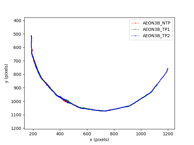
We can see that the trajectories of the three mice are close to a circular arc. Notice that the x and y axes are set to equal scales, and that the origin of the coordinate system is at the top left of the image. This follows the convention for SLEAP and most image processing tools.

We can also color the data points based on their timestamps:

fig, axes = plt.subplots(3, 1, sharey=True)
for mouse_name, ax in zip(position.individuals.values, axes, strict=False):
    sc = ax.scatter(
        position.sel(individuals=mouse_name, space="x"),
        position.sel(individuals=mouse_name, space="y"),
        s=2,
        c=position.time,
        cmap="viridis",
    )
    ax.invert_yaxis()
    ax.set_title(mouse_name)
    ax.set_xlabel("x (pixels)")
    ax.set_ylabel("y (pixels)")
    ax.axis("equal")
    fig.colorbar(sc, ax=ax, label="time (s)")
fig.tight_layout()

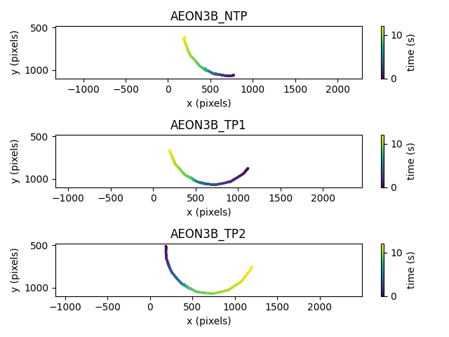
These plots show that for this snippet of the data, two of the mice (AEON3B_NTP and AEON3B_TP1) moved around the circle in clockwise direction, and the third mouse (AEON3B_TP2) followed an anti-clockwise direction.

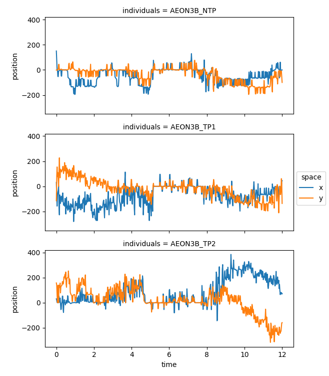
We can also easily plot the components of the position vector against time using xarray’s built-in plotting methods. We use xarray.DataArray.squeeze() to remove the dimension of length 1 from the data (the keypoints dimension).

position.squeeze().plot.line(x="time", row="individuals", aspect=2, size=2.5)
plt.gcf().show()

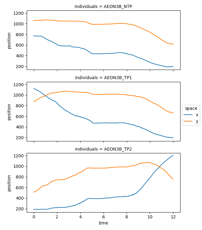
If we use xarray’s plotting function, the axes units are automatically taken from the data array. In our case, time is expressed in seconds, and the x and y coordinates of the position are in pixels.

Compute displacement

The movement.kinematics module provides functions to compute various kinematic quantities, such as displacement, velocity, and acceleration. We can start off by computing the distance travelled by the mice along their trajectories:

import movement.kinematics as kin

displacement = kin.compute_displacement(position)

The movement.kinematics.compute_displacement() function will return a data array equivalent to the position one, but holding displacement data along the space axis, rather than position data.

The displacement data array holds, for a given individual and keypoint at timestep t, the vector that goes from its previous position at time t-1 to its current position at time t.

And what happens at t=0, since there is no previous timestep? We define the displacement vector at time t=0 to be the zero vector. This way the shape of the displacement data array is the same as the position array:

print(f"Shape of position: {position.shape}")
print(f"Shape of displacement: {displacement.shape}")

Shape of position: (601, 2, 1, 3)
Shape of displacement: (601, 2, 1, 3)

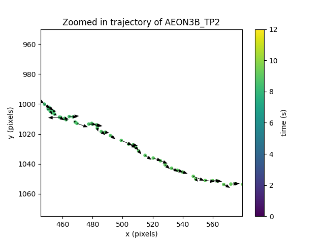
We can visualise these displacement vectors with a quiver plot. In this case we focus on the mouse AEON3B_TP2:

mouse_name = "AEON3B_TP2"

fig = plt.figure()
ax = fig.add_subplot()

# plot position data
sc = ax.scatter(
    position.sel(individuals=mouse_name, space="x"),
    position.sel(individuals=mouse_name, space="y"),
    s=15,
    c=position.time,
    cmap="viridis",
)

# plot displacement vectors: at t, vector from t-1 to t
ax.quiver(
    position.sel(individuals=mouse_name, space="x"),
    position.sel(individuals=mouse_name, space="y"),
    displacement.sel(individuals=mouse_name, space="x"),
    displacement.sel(individuals=mouse_name, space="y"),
    angles="xy",
    scale=1,
    scale_units="xy",
    headwidth=7,
    headlength=9,
    headaxislength=9,
)

ax.axis("equal")
ax.set_xlim(450, 575)
ax.set_ylim(950, 1075)
ax.set_xlabel("x (pixels)")
ax.set_ylabel("y (pixels)")
ax.set_title(f"Zoomed in trajectory of {mouse_name}")
ax.invert_yaxis()
fig.colorbar(sc, ax=ax, label="time (s)")

<matplotlib.colorbar.Colorbar object at 0x7fe08d517b90>

Notice that this figure is not very useful as a visual check: we can see that there are vectors defined for each point in the trajectory, but we have no easy way to verify they are indeed the displacement vectors from t-1 to t.

If instead we plot the opposite of the displacement vector, we will see that at every time t, the vectors point to the position at t-1. Remember that the displacement vector is defined as the vector at time t, that goes from the previous position t-1 to the current position at t. Therefore, the opposite vector will point from the position point at t, to the position point at t-1.

We can easily do this by flipping the sign of the displacement vector in the plot above:

mouse_name = "AEON3B_TP2"

fig = plt.figure()
ax = fig.add_subplot()

# plot position data
sc = ax.scatter(
    position.sel(individuals=mouse_name, space="x"),
    position.sel(individuals=mouse_name, space="y"),
    s=15,
    c=position.time,
    cmap="viridis",
)

# plot displacement vectors: at t, vector from t-1 to t
ax.quiver(
    position.sel(individuals=mouse_name, space="x"),
    position.sel(individuals=mouse_name, space="y"),
    -displacement.sel(individuals=mouse_name, space="x"),  # flipped sign
    -displacement.sel(individuals=mouse_name, space="y"),  # flipped sign
    angles="xy",
    scale=1,
    scale_units="xy",
    headwidth=7,
    headlength=9,
    headaxislength=9,
)
ax.axis("equal")
ax.set_xlim(450, 575)
ax.set_ylim(950, 1075)
ax.set_xlabel("x (pixels)")
ax.set_ylabel("y (pixels)")
ax.set_title(f"Zoomed in trajectory of {mouse_name}")
ax.invert_yaxis()
fig.colorbar(sc, ax=ax, label="time (s)")

<matplotlib.colorbar.Colorbar object at 0x7fe08d579510>

Now we can visually verify that indeed the displacement vector connects the previous and current positions as expected.

With the displacement data we can compute the distance travelled by the mouse along its trajectory.

# length of each displacement vector
displacement_vectors_lengths = compute_norm(
    displacement.sel(individuals=mouse_name)
)

# sum the lengths of all displacement vectors (in pixels)
total_displacement = displacement_vectors_lengths.sum(dim="time").values[0]

print(
    f"The mouse {mouse_name}'s trajectory is {total_displacement:.2f} "
    "pixels long"
)

The mouse AEON3B_TP2's trajectory is 1640.09 pixels long

Compute velocity

We can easily compute the velocity vectors for all individuals in our data array:

velocity = kin.compute_velocity(position)

The movement.kinematics.compute_velocity() function will return a data array equivalent to the position one, but holding velocity data along the space axis, rather than position data. Notice how xarray nicely deals with the different individuals and spatial dimensions for us! ✨

We can plot the components of the velocity vector against time using xarray’s built-in plotting methods. We use xarray.DataArray.squeeze() to remove the dimension of length 1 from the data (the keypoints dimension).

velocity.squeeze().plot.line(x="time", row="individuals", aspect=2, size=2.5)
plt.gcf().show()

The components of the velocity vector seem noisier than the components of the position vector. This is expected, since we are deriving the velocity using differences in position (which is somewhat noisy), over small stepsizes. More specifically, we use numpy’s gradient implementation, which uses second order central differences.

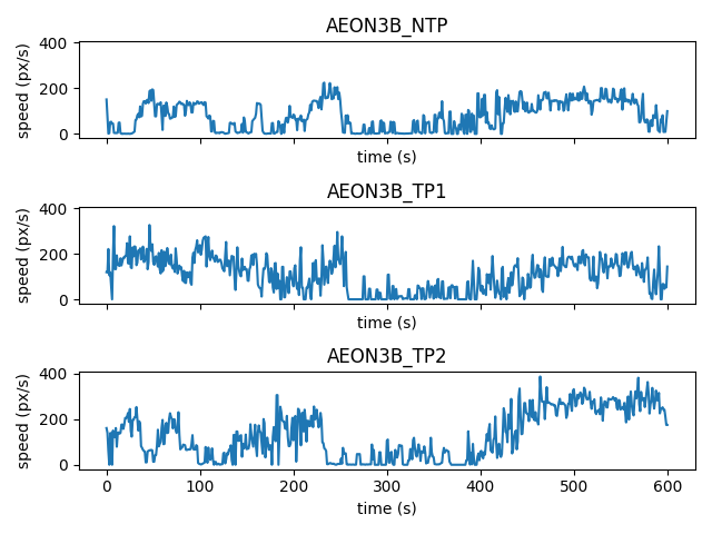
We can also visualise the speed, as the magnitude (norm) of the velocity vector:

fig, axes = plt.subplots(3, 1, sharex=True, sharey=True)
for mouse_name, ax in zip(velocity.individuals.values, axes, strict=False):
    # compute the magnitude of the velocity vector for one mouse
    speed_one_mouse = compute_norm(velocity.sel(individuals=mouse_name))
    # plot speed against time
    ax.plot(speed_one_mouse)
    ax.set_title(mouse_name)
    ax.set_xlabel("time (s)")
    ax.set_ylabel("speed (px/s)")
fig.tight_layout()

To visualise the direction of the velocity vector at each timestep, we can use a quiver plot:

mouse_name = "AEON3B_TP2"
fig = plt.figure()
ax = fig.add_subplot()
# plot trajectory (position data)
sc = ax.scatter(
    position.sel(individuals=mouse_name, space="x"),
    position.sel(individuals=mouse_name, space="y"),
    s=15,
    c=position.time,
    cmap="viridis",
)
# plot velocity vectors
ax.quiver(
    position.sel(individuals=mouse_name, space="x"),
    position.sel(individuals=mouse_name, space="y"),
    velocity.sel(individuals=mouse_name, space="x"),
    velocity.sel(individuals=mouse_name, space="y"),
    angles="xy",
    scale=2,
    scale_units="xy",
    color="r",
)
ax.axis("equal")
ax.set_xlabel("x (pixels)")
ax.set_ylabel("y (pixels)")
ax.set_title(f"Velocity quiver plot for {mouse_name}")
ax.invert_yaxis()
fig.colorbar(sc, ax=ax, label="time (s)")
fig.show()

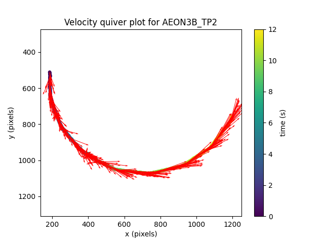
Here we scaled the length of vectors to half of their actual value (scale=2) for easier visualisation.

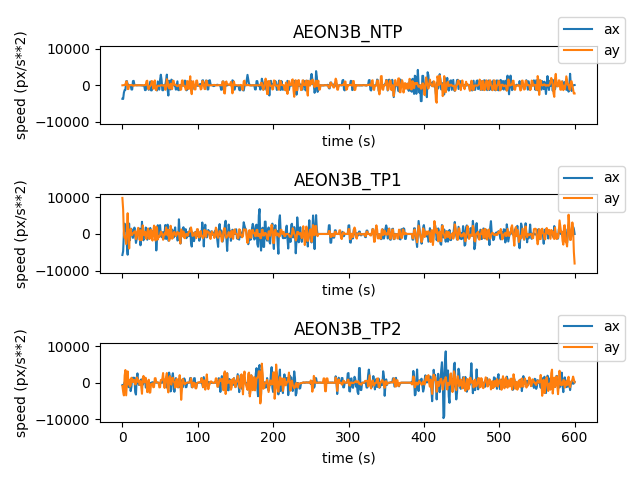
Compute acceleration

Let’s now compute the acceleration for all individuals in our data array:

accel = kin.compute_acceleration(position)

and plot of the components of the acceleration vector ax, ay per individual:

fig, axes = plt.subplots(3, 1, sharex=True, sharey=True)
for mouse_name, ax in zip(accel.individuals.values, axes, strict=False):
    # plot x-component of acceleration vector
    ax.plot(
        accel.sel(individuals=mouse_name, space=["x"]).squeeze(),
        label="ax",
    )
    # plot y-component of acceleration vector
    ax.plot(
        accel.sel(individuals=mouse_name, space=["y"]).squeeze(),
        label="ay",
    )
    ax.set_title(mouse_name)
    ax.set_xlabel("time (s)")
    ax.set_ylabel("speed (px/s**2)")
    ax.legend(loc="center right", bbox_to_anchor=(1.07, 1.07))
fig.tight_layout()

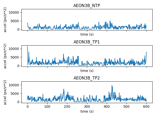
We can also compute and visualise the magnitude (norm) of the acceleration vector for each individual:

fig, axes = plt.subplots(3, 1, sharex=True, sharey=True)
for mouse_name, ax in zip(accel.individuals.values, axes, strict=False):
    # compute magnitude of the acceleration vector for one mouse
    accel_one_mouse = compute_norm(accel.sel(individuals=mouse_name))

    # plot acceleration against time
    ax.plot(accel_one_mouse)
    ax.set_title(mouse_name)
    ax.set_xlabel("time (s)")
    ax.set_ylabel("accel (px/s**2)")
fig.tight_layout()