Compute distances and angles to regions of interest

Compute distances, approach vectors, and both egocentric and allocentric boundary angles relative to regions of interest (RoIs).

Imports

# For interactive plots: install ipympl with `pip install ipympl` and uncomment
# the following lines in your notebook
# %matplotlib widget
import matplotlib.pyplot as plt
import numpy as np
import xarray as xr

from movement import sample_data
from movement.kinematics import compute_velocity
from movement.plots import plot_centroid_trajectory
from movement.roi import PolygonOfInterest

Load sample dataset

In this example, we will use the SLEAP_three-mice_Aeon_proofread example dataset. We only need the position data array, so we store it in a separate variable.

ds = sample_data.fetch_dataset("SLEAP_three-mice_Aeon_proofread.analysis.h5")
positions: xr.DataArray = ds.position

The data we have loaded used an arena setup that we have plotted below.

arena_fig, arena_ax = plt.subplots(1, 1)
# Overlay an image of the experimental arena
arena_image = ds.frame_path
arena_ax.imshow(plt.imread(arena_image))

arena_ax.set_xlabel("x (pixels)")
arena_ax.set_ylabel("y (pixels)")

arena_fig.show()

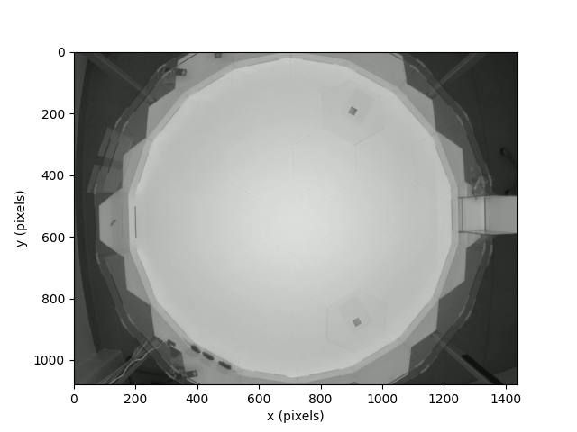
The arena is divided up into three main sub-regions. The cuboidal structure on the right-hand-side of the arena is the nest of the three individuals taking part in the experiment. The majority of the arena is an open octadecagonal (18-sided) shape, which is the bright central region that encompasses most of the image. This central region is surrounded by a (comparatively thin) “ring”, which links the central region to the nest. In this example, we will look at how we can use the functionality for regions of interest (RoIs) provided by movement to analyse our sample dataset.

Define regions of interest

In order to ask questions about the behaviour of our individuals with respect to the arena, we first need to define the RoIs to represent the separate pieces of our arena programmatically. Since each part of our arena is two-dimensional, we will use a PolygonOfInterest to describe each of them.

In the future, the movement plugin for napari will support creating regions of interest by clicking points and drawing shapes in the napari GUI. For the time being, we can still define our RoIs by specifying the points that make up the interior and exterior boundaries. So first, let’s define the boundary vertices of our various regions.

# The centre of the arena is located roughly here
centre = np.array([712.5, 541])
# The "width" (distance between the inner and outer octadecagonal rings) is 40
# pixels wide
ring_width = 40.0
# The distance between opposite vertices of the outer ring is 1090 pixels
ring_extent = 1090.0

# Create the vertices of a "unit" octadecagon, centred on (0,0)
n_pts = 18
unit_shape = np.array(
    [
        np.exp((np.pi / 2.0 + (2.0 * i * np.pi) / n_pts) * 1.0j)
        for i in range(n_pts)
    ],
    dtype=complex,
)
# Then stretch and translate the reference to match our arena
ring_outer_boundary = ring_extent / 2.0 * unit_shape.copy()
ring_outer_boundary = (
    np.array([ring_outer_boundary.real, ring_outer_boundary.imag]).transpose()
    + centre
)
core_boundary = (ring_extent - ring_width) / 2.0 * unit_shape.copy()
core_boundary = (
    np.array([core_boundary.real, core_boundary.imag]).transpose() + centre
)

nest_corners = ((1245, 585), (1245, 475), (1330, 480), (1330, 580))

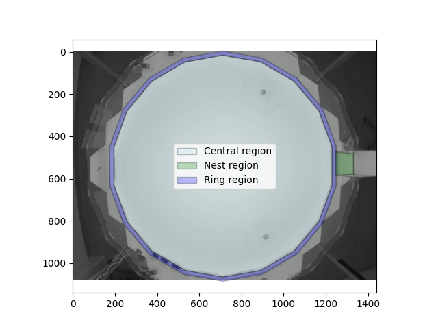
Our central region is a solid shape without any interior holes. To create the appropriate RoI, we just pass the coordinates in either clockwise or counter-clockwise order.

central_region = PolygonOfInterest(core_boundary, name="Central region")

Likewise, the nest is also just a solid shape without any holes. Note that we are only registering the “floor” of the nest here.

nest_region = PolygonOfInterest(nest_corners, name="Nest region")

To create an RoI representing the ring region, we need to provide an interior boundary so that movement knows our ring region has a “hole”. movement’s PolygonsOfInterest can actually support multiple (non-overlapping) holes, which is why the holes argument takes a list.

ring_region = PolygonOfInterest(
    ring_outer_boundary, holes=[core_boundary], name="Ring region"
)

arena_fig, arena_ax = plt.subplots(1, 1)
# Overlay an image of the experimental arena
arena_ax.imshow(plt.imread(arena_image))

central_region.plot(arena_ax, facecolor="lightblue", alpha=0.25)
nest_region.plot(arena_ax, facecolor="green", alpha=0.25)
ring_region.plot(arena_ax, facecolor="blue", alpha=0.25)
arena_ax.legend()
arena_fig.show()

View individual paths inside the arena

We can now overlay the paths that the individuals followed on top of our image of the arena and the RoIs that we have defined.

arena_fig, arena_ax = plt.subplots(1, 1)
# Overlay an image of the experimental arena
arena_ax.imshow(plt.imread(arena_image))

central_region.plot(
    arena_ax, facecolor="lightblue", alpha=0.25, label=central_region.name
)
nest_region.plot(
    arena_ax, facecolor="green", alpha=0.25, label=nest_region.name
)
ring_region.plot(
    arena_ax, facecolor="blue", alpha=0.25, label=ring_region.name
)

# Plot trajectories of the individuals
mouse_names_and_colours = list(
    zip(positions.individuals.values, ["r", "g", "b"], strict=False)
)
for mouse_name, col in mouse_names_and_colours:
    plot_centroid_trajectory(
        positions,
        individual=mouse_name,
        ax=arena_ax,
        linestyle="-",
        marker=".",
        s=1,
        c=col,
        label=mouse_name,
    )
arena_ax.set_title("Individual trajectories within the arena")
arena_ax.legend()

arena_fig.show()

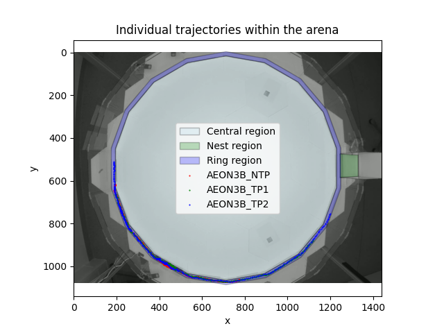
At a glance, it looks like all the individuals remained inside the ring-region for the duration of the experiment. We can verify this programmatically, by asking whether the ring_region contained the individuals’ locations, at all recorded time-points.

# This is a DataArray with dimensions: time, keypoint, and individual.
# The values of the DataArray are True/False values, indicating if at the given
# time, the keypoint of individual was inside ring_region.
individual_was_inside = ring_region.contains_point(positions)
all_individuals_in_ring_at_all_times = individual_was_inside.all()

if all_individuals_in_ring_at_all_times:
    print(
        "All recorded positions, at all times,\n"
        "and for all individuals, were inside ring_region."
    )
else:
    print("At least one position was recorded outside the ring_region.")

All recorded positions, at all times,
and for all individuals, were inside ring_region.

Compute the distance to the nest

Defining RoIs means that we can efficiently extract information from our data that depends on the location or relative position of an individual to an RoI. For example, we might be interested in how the distance between an individual and the nest region changes over the course of the experiment. We can query the nest_region that we created for this information.

# Compute all distances to the nest; for all times, keypoints, and
# individuals.
distances_to_nest = nest_region.compute_distance_to(positions)
distances_fig, distances_ax = plt.subplots(1, 1)
for mouse_name, col in mouse_names_and_colours:
    distances_ax.plot(
        distances_to_nest.sel(individuals=mouse_name),
        c=col,
        label=mouse_name,
    )
distances_ax.legend()
distances_ax.set_xlabel("Time (frames)")
distances_ax.set_ylabel("Distance to nest_region (pixels)")
distances_fig.show()

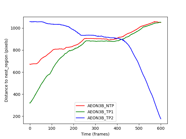
We can see that the AEON38_TP2 individual appears to be moving towards the nest during the experiment, whilst the other two individuals are moving away from the nest. The “plateau” in the figure between frames 200-400 is when the individuals meet in the ring_region, and remain largely stationary in a group until they can pass each other.

One other thing to note is that compute_distance_to is returning the distance “as the crow flies” to the nest_region. This means that structures potentially in the way (such as the ring_region walls) are not accounted for in this distance calculation. Further to this, the “distance to a RoI” should always be understood as “the distance from a point to the closest point within an RoI”.

If we wanted to check the direction of closest approach to a region, referred to as the approach vector, we can use the compute_approach_vector method. The distances that we computed via compute_distance_to are just the magnitudes of the approach vectors.

approach_vectors = nest_region.compute_approach_vector(positions)

The boundary_only keyword

From our plot of the distances to the nest, we saw a time-window in which the individuals are grouped up, possibly trying to pass each other as they approach from different directions. We might be interested in whether they move to opposite walls of the ring while doing so. To examine this, we can plot the distance between each individual and the ring_region, using the same commands as above.

However, we get something slightly unexpected:

distances_to_ring_wall = ring_region.compute_distance_to(positions)
distances_fig, distances_ax = plt.subplots(1, 1)
for mouse_name, col in mouse_names_and_colours:
    distances_ax.plot(
        distances_to_ring_wall.sel(individuals=mouse_name),
        c=col,
        label=mouse_name,
    )
distances_ax.legend()
distances_ax.set_xlabel("Time (frames)")
distances_ax.set_ylabel("Distance to closest ring_region wall (pixels)")

print(
    "distances_to_ring_wall are all zero:",
    np.allclose(distances_to_ring_wall, 0.0),
)

distances_fig.show()

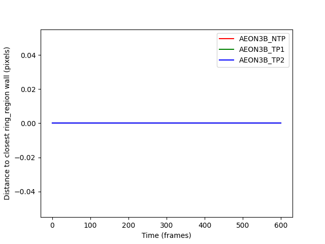
distances_to_ring_wall are all zero: True

The distances are all zero because when a point is inside a region, the closest point to it is itself.

To find distances to the ring’s walls instead, we can use boundary_only=True, which tells movement to only look at points on the boundary of the region, not inside it. Note that for 1D regions (LineOfInterest), the “boundary” is just the endpoints of the line.

Let’s try again with boundary_only=True:

distances_to_ring_wall = ring_region.compute_distance_to(
    positions, boundary_only=True
)
distances_fig, distances_ax = plt.subplots(1, 1)
for mouse_name, col in mouse_names_and_colours:
    distances_ax.plot(
        distances_to_ring_wall.sel(individuals=mouse_name),
        c=col,
        label=mouse_name,
    )
distances_ax.legend()
distances_ax.set_xlabel("Time (frames)")
distances_ax.set_ylabel("Distance to closest ring_region wall (pixels)")

print(
    "distances_to_ring_wall are all zero:",
    np.allclose(distances_to_ring_wall, 0.0),
)

distances_fig.show()

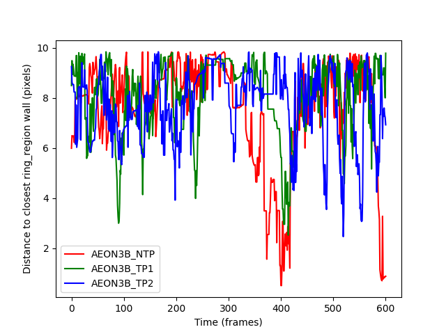
distances_to_ring_wall are all zero: False

The resulting plot looks much more like what we expect, but is again not very helpful; we get the distance to the closest point on either the interior or exterior wall of the ring_region. This means that we can’t tell if the individuals do move to opposite walls when passing each other. Instead, let’s ask for the distance to just the exterior wall.

# Note that the exterior_boundary of the ring_region is a 1D RoI (a series of
# connected line segments). As such, boundary_only needs to be False.
distances_to_exterior = ring_region.exterior_boundary.compute_distance_to(
    positions
)
distances_exterior_fig, distances_exterior_ax = plt.subplots(1, 1)
for mouse_name, col in mouse_names_and_colours:
    distances_exterior_ax.plot(
        distances_to_exterior.sel(individuals=mouse_name),
        c=col,
        label=mouse_name,
    )
distances_exterior_ax.legend()
distances_exterior_ax.set_xlabel("Time (frames)")
distances_exterior_ax.set_ylabel("Distance to exterior wall (pixels)")
distances_exterior_fig.show()

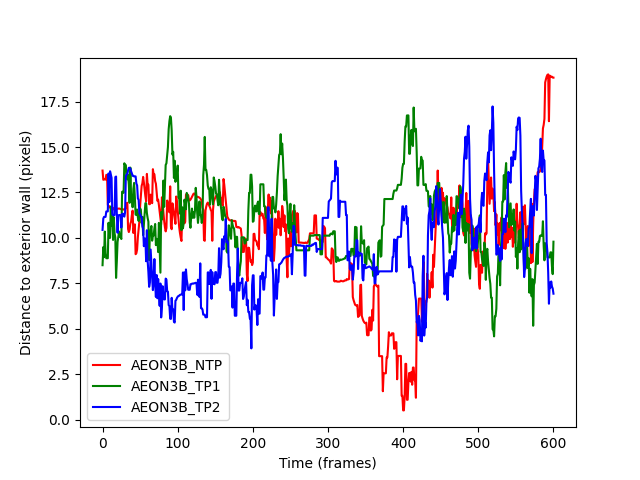
This output is much more helpful. We see that the individuals are largely the same distance from the exterior wall during frames 250-350, and then notice that;

• Individual AEON_TP1 moves far away from the exterior wall,

• AEON3B_NTP moves almost up to the exterior wall,

• and AEON3B_TP2 seems to remain between the other two individuals.

After frame 400, the individuals appear to go back to chaotic distances from the exterior wall again, which is consistent with them having passed each other in the ring_region and once again having the entire width of the ring to explore.

Boundary angles

Having observed the individuals’ behaviour as they pass one another in the ring_region, we can begin to ask questions about their orientation with respect to the nest. movement currently supports the computation of two such “boundary angles”;

• The allocentric boundary angle. Given a region of interest \(R\), reference vector \(\vec{r}\) (such as global north), and a position \(p\) in space (e.g. the position of an individual), the allocentric boundary angle is the signed angle between the approach vector from \(p\) to \(R\), and \(\vec{r}\).

• The egocentric boundary angle. Given a region of interest \(R\), a forward vector \(\vec{f}\) (e.g. the direction of travel of an individual), and the point of origin of \(\vec{f}\) denoted \(p\) (e.g. the individual’s current position), the egocentric boundary angle is the signed angle between the approach vector from \(p\) to \(R\), and \(\vec{f}\).

Note that egocentric angles are generally computed with changing frames of reference in mind - the forward vector may be varying in time as the individual moves around the arena. By contrast, allocentric angles are always computed with respect to some fixed reference frame.

For the purposes of our example, we will define our “forward vector” as the velocity vector between successive time-points, for each individual - we can compute this from positions using the compute_velocity function in movement.kinematics. We will also define our reference frame, or “global north” direction, to be the direction of the positive x-axis.

forward_vector = compute_velocity(positions)
global_north = np.array([1.0, 0.0])

allocentric_angles = nest_region.compute_allocentric_angle_to_nearest_point(
    positions,
    reference_vector=global_north,
    in_degrees=True,
)
egocentric_angles = nest_region.compute_egocentric_angle_to_nearest_point(
    forward_vector,
    positions[:-1],
    in_degrees=True,
)

angle_plot, angle_ax = plt.subplots(2, 1, sharex=True)
allo_ax, ego_ax = angle_ax

for mouse_name, col in mouse_names_and_colours:
    allo_ax.plot(
        allocentric_angles.sel(individuals=mouse_name),
        c=col,
        label=mouse_name,
    )
    ego_ax.plot(
        egocentric_angles.sel(individuals=mouse_name),
        c=col,
        label=mouse_name,
    )

ego_ax.set_xlabel("Time (frames)")

ego_ax.set_ylabel("Egocentric angle (degrees)")
allo_ax.set_ylabel("Allocentric angle (degrees)")
allo_ax.legend()

angle_plot.tight_layout()
angle_plot.show()

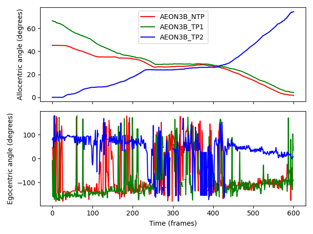
Allocentric angles show step-like behaviour because they only depend on an individual’s position relative to the RoI, not their forward vector. This makes the allocentric angle graph resemble the distance-to-nest graph (inverted on the y-axis), with a “plateau” during frames 200-400 when the individuals are (largely) stationary while passing each other.

Egocentric angles, on the other hand, fluctuate more due to their sensitivity to changes in the forward vector. Outside frames 200-400, we see trends:

• AEON3B_TP2 moves clockwise around the ring, so its egocentric angle decreases ever so slightly with time - almost hitting an angle of 0 degrees as it moves along the direction of closest approach after passing the other individuals.

• The other two individuals move counter-clockwise, so their angles show a gradual increase with time. Because the two individuals occasionally get in each others’ way, we see frequent “spikes” in their egocentric angles as their forward vectors rapidly change.

During frames 200-400, rapid changes in direction cause large fluctuations in the egocentric angles of all the individuals, reflecting the individuals’ attempts to avoid colliding with (and to make space to move passed) each other.