Pupil tracking

Look at eye movements and pupil diameter.

Imports

import sleap_io as sio
import xarray as xr
from matplotlib import pyplot as plt

import movement.kinematics as kin
from movement import sample_data
from movement.filtering import rolling_filter
from movement.plots import plot_centroid_trajectory

Load the data

We will use two datasets from the sample data module. These datasets involve recordings of the eyes of mice placed on a rotating platform with different visual stimuli. The uniform condition features a uniformly lit surround stimulus, whereas the black condition was acquired in the dark. These datasets were tracked using DeepLabCut (DLC) and include four keypoints: two on either side of the pupil (pupil-L and pupil-R) and two on either side of the eye (eye-L and eye-R).

ds_black = sample_data.fetch_dataset(
    "DLC_rotating-mouse_eye-tracking_stim-black.predictions.h5",
    with_video=True,
)
ds_uniform = sample_data.fetch_dataset(
    "DLC_rotating-mouse_eye-tracking_stim-uniform.predictions.h5",
    with_video=True,
)
# Save data in a dictionary.
ds_dict = {"black": ds_black, "uniform": ds_uniform}

Print the content of one of the datasets.

print(ds_dict["black"])

<xarray.Dataset> Size: 728kB
Dimensions:      (time: 7000, space: 2, keypoints: 4, individuals: 1)
Coordinates:
  * time         (time) float64 56kB 0.0 0.025 0.05 0.075 ... 174.9 174.9 175.0
  * space        (space) <U1 8B 'x' 'y'
  * keypoints    (keypoints) <U7 112B 'pupil-L' 'pupil-R' 'eye-L' 'eye-R'
  * individuals  (individuals) <U12 48B 'individual_0'
Data variables:
    position     (time, space, keypoints, individuals) float64 448kB 258.8 .....
    confidence   (time, keypoints, individuals) float64 224kB 1.0 1.0 ... 1.0
Attributes:
    source_software:  DeepLabCut
    ds_type:          poses
    fps:              40.0
    time_unit:        seconds
    source_file:      /home/runner/.movement/data/poses/DLC_rotating-mouse_ey...
    frame_path:       /home/runner/.movement/data/frames/rotating-mouse_eye-t...
    video_path:       /home/runner/.movement/data/videos/rotating-mouse_eye-t...

Explore the accompanying videos

for ds_name, ds in ds_dict.items():
    video = sio.load_video(ds.video_path)
    # To avoid having to reload the video again we add it to ds as attribute
    ds_dict[ds_name] = ds.assign_attrs({"video": video})
    n_frames, height, width, channels = video.shape
    print(f"Dataset: {ds_name}")
    print(f"Number of frames: {n_frames}")
    print(f"Frame size: {width}x{height}")
    print(f"Number of channels: {channels}\n")

Dataset: black
Number of frames: 7000
Frame size: 640x480
Number of channels: 1

Dataset: uniform
Number of frames: 7000
Frame size: 640x480
Number of channels: 1

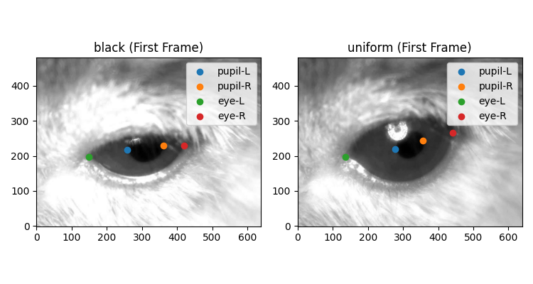
Plot first frame with keypoints

fig, ax = plt.subplots(1, 2, figsize=(7.5, 4))
for i, (da_name, ds) in enumerate(ds_dict.items()):
    ax[i].imshow(ds.video[0], cmap="gray")  # plot first video frame
    for keypoint in ds.keypoints.values:
        x = ds.position.sel(time=0, space="x", keypoints=keypoint)
        y = ds.position.sel(time=0, space="y", keypoints=keypoint)
        ax[i].scatter(x, y, label=keypoint)  # plot keypoints
    ax[i].legend()
    ax[i].set_title(f"{da_name} (First Frame)")
    ax[i].invert_yaxis()  # because the dataset was collected flipped
plt.tight_layout()
plt.show()

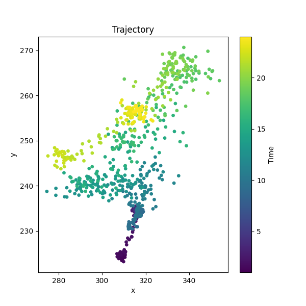
Pupil trajectory

A quick plot of the trajectory of the centre of the pupil using the plot_centroid_trajectory function from movement.plots.

time_window = slice(1, 24)  # seconds
position_black = ds_black.position.sel(time=time_window)  # data array to plot
fig, ax = plot_centroid_trajectory(
    position_black, keypoints=["pupil-L", "pupil-R"]
)
fig.show()

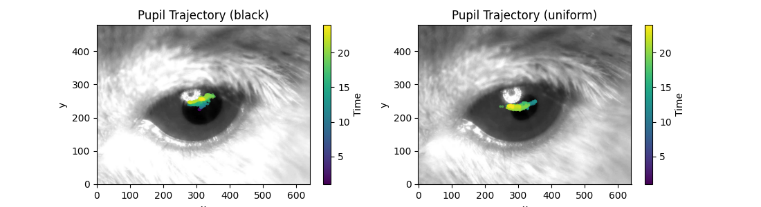
Pupil trajectories on top of video frame

We can look at pupil trajectories plotted on top of a video frame.

fig, ax = plt.subplots(1, 2, figsize=(11, 3))
for i, (ds_name, ds) in enumerate(ds_dict.items()):
    ax[i].imshow(ds.video[100], cmap="gray")  # Plot frame 100 as background
    plot_centroid_trajectory(
        ds.position.sel(time=time_window),  # Select time window
        ax=ax[i],
        keypoints=["pupil-L", "pupil-R"],
        alpha=0.5,
        s=3,
    )
    ax[i].invert_yaxis()
    ax[i].set_title(f"Pupil Trajectory ({ds_name})")
fig.show()

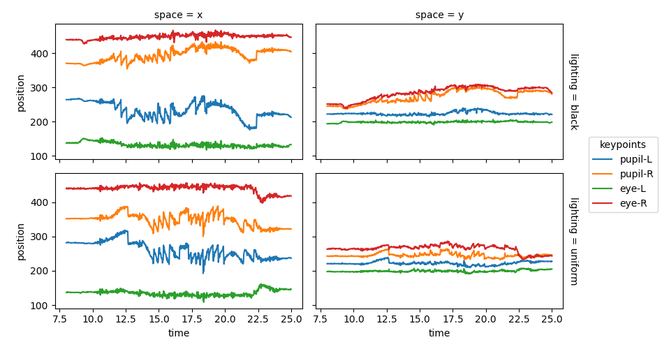
Keypoint positions over time

For the rest of this example we are only interested in the position data. For convenience, We will combine the two position arrays into a single array with a new dimension called lighting.

positions = xr.concat([ds_black.position, ds_uniform.position], "lighting")
positions.coords["lighting"] = ["black", "uniform"]

Define plotting parameters for reuse.

plot_params = {
    "x": "time",
    "hue": "keypoints",
    "col": "space",
    "row": "lighting",
    "aspect": 1.5,
    "size": 2.5,
}
sel = {"time": slice(8, 25)}

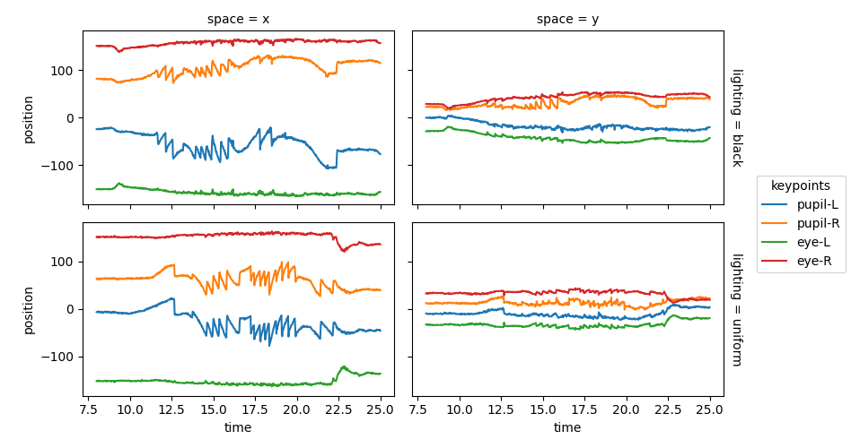
Plot the keypoint positions over time.

positions.sel(**sel).squeeze().plot.line(**plot_params)
plt.subplots_adjust(right=0.85)  # Make space on the right for the legend
plt.show()

Normalised keypoint positions over time

Normalizing the pupil’s position relative to the midpoint of the eye reduces the impact of head movements or artefacts caused by camera movement. By subtracting the position of the eye’s midpoint, we effectively transform the data into a moving coordinate system, with the eye’s midpoint as the origin. In the rest of the example, the normalised data will be used.

eye_midpoint = positions.sel(keypoints=["eye-L", "eye-R"]).mean("keypoints")
positions_norm = positions - eye_midpoint

We plot the x and y positions again, but now using the normalised data.

positions_norm.sel(**sel).squeeze().plot.line(**plot_params)
plt.subplots_adjust(right=0.85)
plt.show()

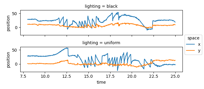
Pupil position over time

To look at pupil position—and later also velocity—over time, we use the pupil centroid (in this case the midpoint between keypoints pupil-L and pupil-R). The keypoint pupil-C is assigned using xarray.DataArray.assign_coords.

pupil_centroid = (
    positions_norm.sel(keypoints=["pupil-L", "pupil-R"])
    .mean("keypoints")
    .assign_coords({"keypoints": "pupil-C"})
)

The pupil centroid keypoint pupil-C is be added to the positions_norm using xarray.concat.

positions_norm = xr.concat([positions_norm, pupil_centroid], dim="keypoints")

Now the position of the pupil centroid pupil-C can be plotted.

positions_norm.sel(keypoints="pupil-C", **sel).squeeze().plot.line(
    x="time", hue="space", row="lighting", aspect=3.5, size=1.5
)
plt.show()

Pupil velocity over time

In these experiments, the mouse is being rotated clock- or anti-clock-wise, triggering the vestibulo-ocular reflex. This reflex involves the vestibular system in the inner ear, that detects head motion and adjusts eye position to maintain stable vision.

When the head turns beyond the range that the vestibulo-ocular reflex can compensate for, a quick, ballistic eye movement is triggered to shift gaze to a new fixation point. These fast eye movements are seen in the previous plot but become even more obvious when the velocity of the pupil centroid is plotted. To do this, we use compute_velocity from the movement.kinematics module to calculate the velocity of the eye movements.

pupil_velocity = kin.compute_velocity(positions_norm.sel(keypoints="pupil-C"))
pupil_velocity.name = "pupil velocity"
pupil_velocity.sel(**sel).squeeze().plot.line(
    x="time", hue="space", row="lighting", aspect=3.5, size=1.5
)
plt.show()

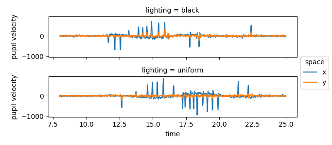
The positive peaks correspond to rapid eye movements to the right, the negative peaks correspond to rapid eye movements to the left.

Pupil diameter

Here we define the pupil diameter as the distance between the two pupil keypoints. We use compute_pairwise_distances from movement.kinematics to calculate the Euclidean distance between pupil-L and pupil-R.

pupil_diameter: xr.DataArray = kin.compute_pairwise_distances(
    positions_norm, dim="keypoints", pairs={"pupil-L": "pupil-R"}
)
pupil_diameter.name = "pupil diameter"

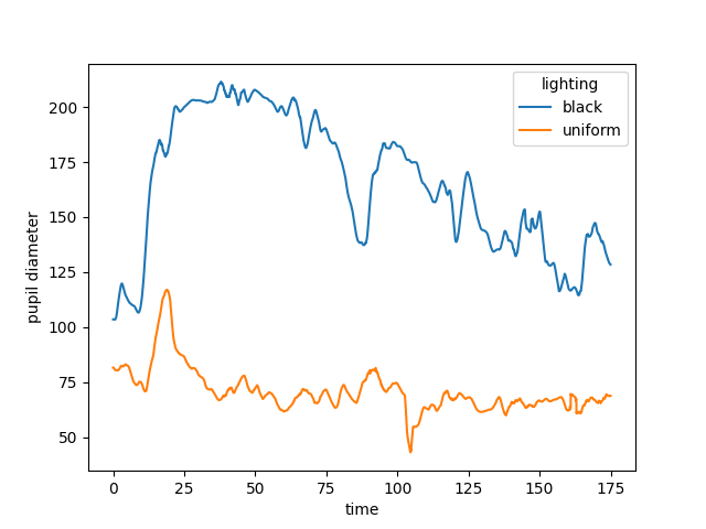
Now the pupil diameter can be plotted.

pupil_diameter.plot.line(x="time", hue="lighting")
plt.show()

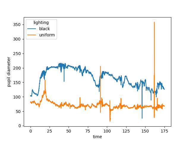
The plot of the pupil diameter looks noisy. The very steep peaks are unlikely to represent real changes in the pupil size. In fact, these steep peaks are probably caused by tracking errors during blinking or squinting. By looking at the distance between the two eye keypoints we can get an idea of whether (and when) the animal is blinking or squinting.

distance_between_eye_keypoints: xr.DataArray = kin.compute_pairwise_distances(
    positions_norm, dim="keypoints", pairs={"eye-L": "eye-R"}
)
distance_between_eye_keypoints.name = "distance (eye-L - eye-R)"

# Combine the datasets into one DataArray
combined = xr.concat(
    [distance_between_eye_keypoints, pupil_diameter], dim="variable"
)
combined = combined.assign_coords(
    variable=["distance (eye-L - eye-R)", "pupil diameter"]
)

# Plot the distance between the eye keypoints alongside the pupil diameter
combined.plot.line(
    x="time", row="lighting", hue="variable", figsize=(8, 4), add_legend=False
)
labels = combined.coords["variable"].values
plt.legend(labels, loc="center", bbox_to_anchor=(0.5, 1.4), ncol=2)
plt.xlabel("time (s)")
[ax.set_ylabel("distance (pixels)") for ax in plt.gcf().axes]
plt.show()

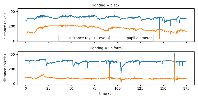
We indeed see that the sharp peaks in pupil diameter correspond to abrupt changes of distance between the two eye keypoints. Compared to fast eye movements and blinking, changes in pupil size are slow. Filters can be applied to reduce noise and make underlying trends in pupil diameter clearer.

Smooth pupil diameter

A rolling mean (moving average) filter is used here to smooth the data by averaging a specified number of data points (window_len). We achieve this by calling the movement.filtering.rolling_filter() function with the statistic="mean" option.

window_len = 80
mean_filter = rolling_filter(
    pupil_diameter, window=window_len, statistic="mean"
)

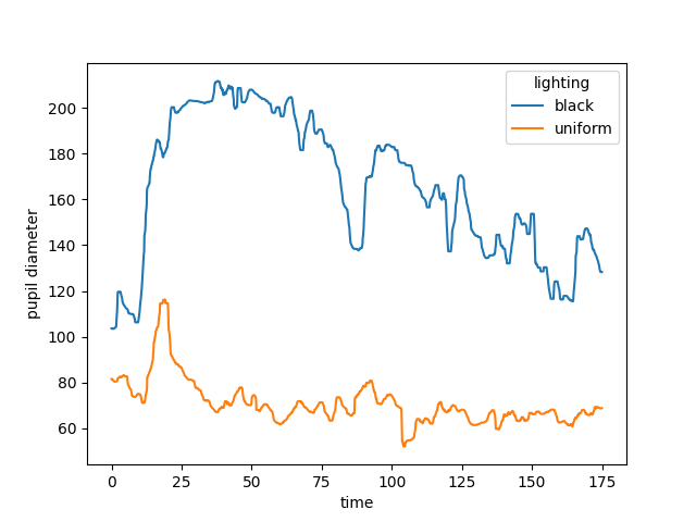
Now the filtered pupil diameter can be plotted.

mean_filter.plot.line(x="time", hue="lighting")
plt.show()

Instead of the mean, we could also use the median, which is the default option for the statistic argument, and should be more robust to outliers.

mdn_filter = rolling_filter(pupil_diameter, window_len, statistic="median")
mdn_filter.plot.line(x="time", hue="lighting")
plt.show()

See also

Smooth pose tracks example.