Load and explore pose tracks

Load and explore an example dataset of pose tracks.

Imports

from matplotlib import pyplot as plt

from movement import sample_data
from movement.io import load_poses

Define the file path

This should be a file output by one of our supported pose estimation frameworks (e.g., DeepLabCut, SLEAP), containing predicted pose tracks. For example, the path could be something like:

# uncomment and edit the following line to point to your own local file
# file_path = "/path/to/my/data.h5"

For the sake of this example, we will use the path to one of the sample datasets provided with movement.

file_path = sample_data.fetch_dataset_paths(
    "SLEAP_three-mice_Aeon_proofread.analysis.h5"
)["poses"]
print(file_path)

/home/runner/.movement/data/poses/SLEAP_three-mice_Aeon_proofread.analysis.h5

Load the data into movement

ds = load_poses.from_sleap_file(file_path, fps=50)
print(ds)

<xarray.Dataset> Size: 27kB
Dimensions:      (time: 601, individuals: 3, keypoints: 1, space: 2)
Coordinates:
  * time         (time) float64 5kB 0.0 0.02 0.04 0.06 ... 11.96 11.98 12.0
  * individuals  (individuals) <U10 120B 'AEON3B_NTP' 'AEON3B_TP1' 'AEON3B_TP2'
  * keypoints    (keypoints) <U8 32B 'centroid'
  * space        (space) <U1 8B 'x' 'y'
Data variables:
    position     (time, individuals, keypoints, space) float32 14kB 770.3 ......
    confidence   (time, individuals, keypoints) float32 7kB nan nan ... nan nan
Attributes:
    fps:              50.0
    time_unit:        seconds
    source_software:  SLEAP
    source_file:      /home/runner/.movement/data/poses/SLEAP_three-mice_Aeon...

The loaded dataset contains two data variables: position and confidence. To get the position data:

position = ds.position

Select and plot data with xarray

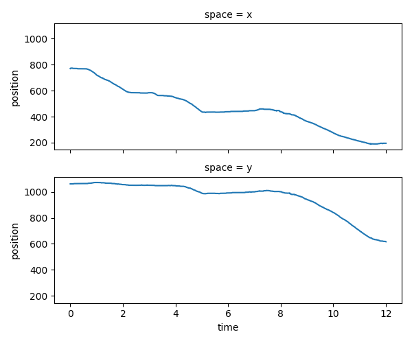
You can use the sel method to index into xarray objects. For example, we can get a DataArray containing only data for a single keypoint of the first individual:

da = position.sel(individuals="AEON3B_NTP", keypoints="centroid")
print(da)

<xarray.DataArray 'position' (time: 601, space: 2)> Size: 5kB
770.3 1.062e+03 773.3 1.062e+03 773.3 ... 618.6 194.6 618.4 194.6 616.4
Coordinates:
  * time         (time) float64 5kB 0.0 0.02 0.04 0.06 ... 11.96 11.98 12.0
    individuals  <U10 40B 'AEON3B_NTP'
    keypoints    <U8 32B 'centroid'
  * space        (space) <U1 8B 'x' 'y'

We could plot the x, y coordinates of this keypoint over time, using xarray’s built-in plotting methods:

da.plot.line(x="time", row="space", aspect=2, size=2.5)

<xarray.plot.facetgrid.FacetGrid object at 0x7fca875b7310>

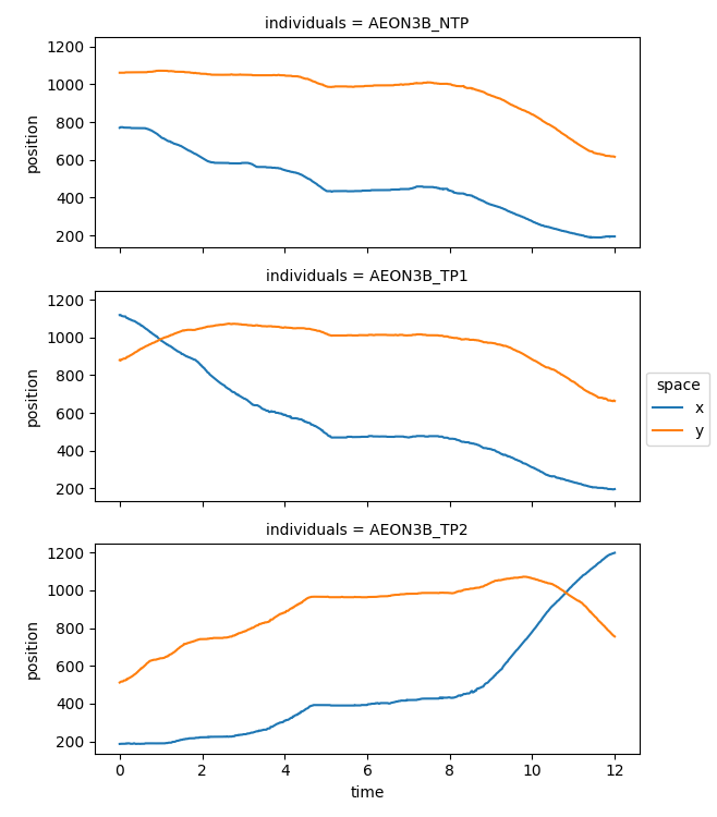
Similarly we could plot the same keypoint’s x, y coordinates for all individuals:

da = position.sel(keypoints="centroid")
da.plot.line(x="time", row="individuals", aspect=2, size=2.5)

<xarray.plot.facetgrid.FacetGrid object at 0x7fca87707d10>

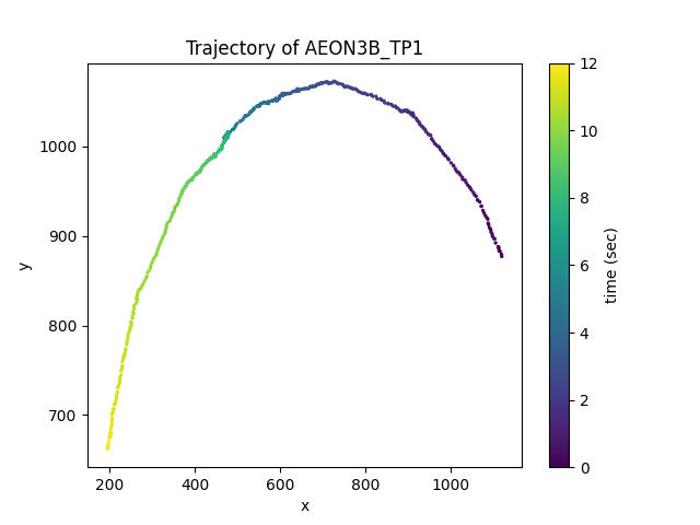
Trajectory plots

We are not limited to xarray’s built-in plots. For example, we can use matplotlib to plot trajectories (using scatter plots):

mouse_name = "AEON3B_TP1"

plt.scatter(
    da.sel(individuals=mouse_name, space="x"),
    da.sel(individuals=mouse_name, space="y"),
    s=2,
    c=da.time,
    cmap="viridis",
)
plt.title(f"Trajectory of {mouse_name}")
plt.xlabel("x")
plt.ylabel("y")
plt.colorbar(label="time (sec)")

<matplotlib.colorbar.Colorbar object at 0x7fca8511cdd0>