Load and upsample bounding boxes tracks

Load bounding boxes tracks and upsample them to match the video frame rate.

Imports

# For interactive plots: install ipympl with `pip install ipympl` and uncomment
# the following line in your notebook
# %matplotlib widget
import csv
import math
import os

import sleap_io as sio
from matplotlib import pyplot as plt

from movement import sample_data
from movement.filtering import interpolate_over_time
from movement.io import load_bboxes

Load sample dataset

In this tutorial, we will use a sample bounding boxes dataset with a single individual (a crab). The clip is part of the Moving Camouflaged Animals Dataset (MoCA) dataset.

We will also download the associated video for visualising the data later.

dataset_dict = sample_data.fetch_dataset_paths(
    "VIA_single-crab_MOCA-crab-1.csv",
    with_video=True,  # download associated video
)

file_path = dataset_dict["bboxes"]
print(file_path)

ds = load_bboxes.from_via_tracks_file(
    file_path, use_frame_numbers_from_file=True
)

/home/runner/.movement/data/bboxes/VIA_single-crab_MOCA-crab-1.csv

The loaded dataset is made up of three data arrays: position, shape, and confidence.

print(ds)

<xarray.Dataset> Size: 2kB
Dimensions:      (time: 35, space: 2, individuals: 1)
Coordinates:
  * time         (time) int64 280B 0 5 10 15 20 25 ... 145 150 155 160 165 167
  * space        (space) <U1 8B 'x' 'y'
  * individuals  (individuals) <U4 16B 'id_1'
Data variables:
    position     (time, space, individuals) float64 560B 1.118e+03 ... 401.9
    shape        (time, space, individuals) float64 560B 320.1 153.2 ... 120.1
    confidence   (time, individuals) float64 280B nan nan nan ... nan nan nan
Attributes:
    fps:              None
    time_unit:        frames
    source_software:  VIA-tracks
    source_file:      /home/runner/.movement/data/bboxes/VIA_single-crab_MOCA...
    ds_type:          bboxes

We can see that the coordinates in the time dimension are expressed in frames, and that we only have data for 1 in 5 frames of the video, plus the last frame (frame number 167).

print(ds.time)

<xarray.DataArray 'time' (time: 35)> Size: 280B
0 5 10 15 20 25 30 35 40 45 50 ... 120 125 130 135 140 145 150 155 160 165 167
Coordinates:
  * time     (time) int64 280B 0 5 10 15 20 25 30 ... 145 150 155 160 165 167

In the following sections of the notebook we will explore options to upsample the dataset by filling in values for the video frames with no data.

Inspect associated video

The video associated to the data contains all 168 frames.

video_path = dataset_dict["video"]

video = sio.load_video(video_path)
n_frames, height, width, channels = video.shape

print(f"Number of frames: {n_frames}")
print(f"Frame size: {width}x{height}")
print(f"Number of channels: {channels}")

Number of frames: 168
Frame size: 1280x720
Number of channels: 3

Let’s inspect the first 6 frames of the video for which we have annotations, and plot the annotated bounding box and centroid at each frame.

# set last frame to plot
end_frame_idx = 25
# create list of frames to loop over with step=5
list_frames = list(range(0, end_frame_idx + 1, 5))

# initialise figure
fig = plt.figure(figsize=(8, 8))  # width, height

# loop over selected frames and plot the data
for i, frame_idx in enumerate(list_frames):
    # add subplot axes
    ax = plt.subplot(math.ceil(len(list_frames) / 2), 2, i + 1)

    # plot frame
    ax.imshow(video[frame_idx])

    # plot box at this frame
    top_left_corner = (
        ds.position.sel(time=frame_idx).data
        - ds.shape.sel(time=frame_idx).data / 2
    ).squeeze()

    bbox = plt.Rectangle(
        xy=tuple(top_left_corner),
        width=ds.shape.sel(time=frame_idx, space="x").item(),
        height=ds.shape.sel(time=frame_idx, space="y").item(),
        edgecolor="red",
        facecolor="none",
        linewidth=1.5,
        label="current frame",
    )
    ax.add_patch(bbox)

    # plot box's centroid at this frame with red ring
    ax.scatter(
        x=ds.position.sel(time=frame_idx, space="x"),
        y=ds.position.sel(time=frame_idx, space="y"),
        s=15,
        color="red",
    )

    # plot past centroid positions in blue
    if frame_idx > 0:
        ax.scatter(
            x=ds.position.sel(time=slice(0, frame_idx - 1), space="x"),
            y=ds.position.sel(time=slice(0, frame_idx - 1), space="y"),
            s=10,
            color="tab:blue",
            label="past frames",
        )

    # plot future centroid positions in white
    ax.scatter(
        x=ds.position.sel(time=slice(frame_idx + 1, end_frame_idx), space="x"),
        y=ds.position.sel(time=slice(frame_idx + 1, end_frame_idx), space="y"),
        s=10,
        color="white",
        label="future frames",
    )

    # set title and labels
    ax.set_title(f"Frame {frame_idx}")
    ax.set_xlabel("x (pixles)")
    ax.set_ylabel("y (pixels)")
    ax.set_xlabel("")
    if frame_idx == 1:
        ax.legend()

fig.tight_layout()

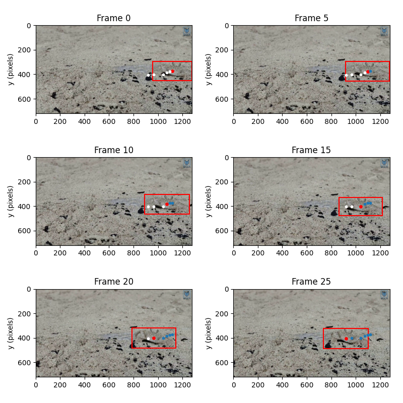
We used xarray’s .sel() method to select the data for the relevant frames directly.

The centroid at each frame is marked with a red marker. The past centroid positions are shown in blue and the future centroid positions in white. Note that in this case the camera is not static relative to the environment.

Fill in empty values with forward filling

We can fill in the frames with empty values for the position and shape arrays by taking the last valid value in time. In this way, a box’s position and shape stay constant if for a current frame the box has no annotation defined.

ds_ff = ds.reindex(
    {"time": list(range(ds.time[-1].item() + 1))},
    method="ffill",  # propagate last valid index value forward
)

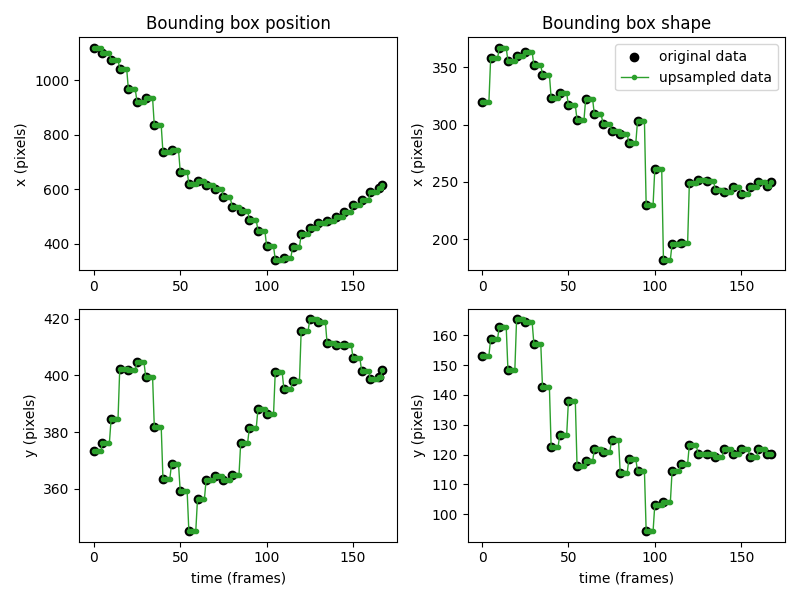
We can verify with a plot that the empty values have been filled in using the last valid value in time.

For this we define a convenience function to plot the x and y coordinates of the position and shape arrays, for the input dataset and for a filled one.

def plot_position_and_shape_xy_coords(ds_input_data, ds_filled, color_filled):
    """Compare the x and y coordinates of the position and shape arrays in time
    for the input and filled datasets.
    """
    fig, axs = plt.subplots(2, 2, figsize=(8, 6))
    for row in range(axs.shape[0]):
        space_coord = ["x", "y"][row]
        for col in range(axs.shape[1]):
            ax = axs[row, col]
            data_array_str = ["position", "shape"][col]

            # plot original data
            ax.scatter(
                x=ds_input_data.time,
                y=ds_input_data[data_array_str].sel(
                    individuals="id_1", space=space_coord
                ),
                marker="o",
                color="black",
                label="original data",
            )

            # plot forward filled data
            ax.plot(
                ds_filled.time,
                ds_filled[data_array_str].sel(
                    individuals="id_1", space=space_coord
                ),
                marker=".",
                linewidth=1,
                color=color_filled,
                label="upsampled data",
            )

            # set axes labels and legend
            ax.set_ylabel(f"{space_coord} (pixels)")
            if row == 0:
                ax.set_title(f"Bounding box {data_array_str}")
                if col == 1:
                    ax.legend()
            if row == 1:
                ax.set_xlabel("time (frames)")

    fig.tight_layout()

In the plot below, the original position and shape data is shown in black, while the forward-filled values are shown in green.

plot_position_and_shape_xy_coords(
    ds, ds_filled=ds_ff, color_filled="tab:green"
)

Fill in empty values with NaN

Alternatively, we can fill in the empty frames with NaN values. This can be useful if we want to interpolate later.

ds_nan = ds.reindex(
    {"time": list(range(ds.time[-1].item() + 1))},
    method=None,  # default
)

Like before, we can verify with a plot that the empty values have been filled with NaN values.

plot_position_and_shape_xy_coords(
    ds, ds_filled=ds_nan, color_filled="tab:blue"
)

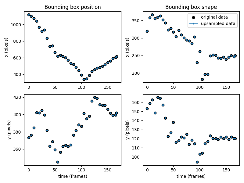
We can further confirm we have NaNs where expected by printing the first few frames of the data.

print("Position data array (first 10 frames):")
print(ds_nan.position.isel(time=slice(0, 10), individuals=0).data)
print("----")
print("Shape data array (first 10 frames):")
print(ds_nan.shape.isel(time=slice(0, 10), individuals=0).data)

Position data array (first 10 frames):
[[1117.895   373.3035]
 [      nan       nan]
 [      nan       nan]
 [      nan       nan]
 [      nan       nan]
 [1098.141   376.1255]
 [      nan       nan]
 [      nan       nan]
 [      nan       nan]
 [      nan       nan]]
----
Shape data array (first 10 frames):
[[320.09  153.191]
 [    nan     nan]
 [    nan     nan]
 [    nan     nan]
 [    nan     nan]
 [357.984 158.835]
 [    nan     nan]
 [    nan     nan]
 [    nan     nan]
 [    nan     nan]]

Linearly interpolate NaN values

We can instead fill in the empty values in the dataset by linearly interpolating the position and shape data arrays. In this way, we would be assuming that the centroid of the bounding box moves linearly between the two annotated values, and its width and height change linearly as well.

We use the dataset with NaN values as an input to the interpolate_over_time function.

ds_interp = ds_nan.copy()

for data_array_str in ["position", "shape"]:
    ds_interp[data_array_str] = interpolate_over_time(
        data=ds_interp[data_array_str],
        method="linear",
        max_gap=None,
        print_report=False,
    )

Like before, we can visually check that the empty data has been imputed as expected by plotting the x and y coordinates of the position and shape arrays in time.

plot_position_and_shape_xy_coords(
    ds, ds_filled=ds_interp, color_filled="tab:orange"
)

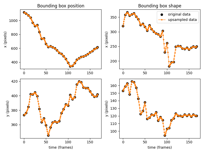
The plot above shows that between the original data points (in black), the data is assumed to evolve linearly (in orange).

Compare methods

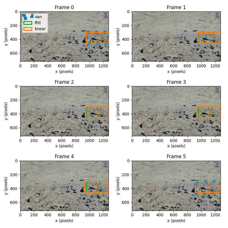
We can now qualitatively compare the bounding boxes computed with the three different filling methods we have seen: forward filling, NaN filling and linear interpolation

In the plot below, the NaN-filled data are plotted in blue, the forward filled values are plotted in orange, and the linearly interpolated values are shown in green.

# initialise figure
fig = plt.figure(figsize=(8, 8))

list_colors = ["tab:blue", "tab:green", "tab:orange"]

# loop over frames
for frame_idx in range(6):
    # add subplot axes
    ax = plt.subplot(3, 2, frame_idx + 1)

    # plot frame
    ax.imshow(video[frame_idx])

    # plot bounding box for each dataset
    for ds_i, ds_filled in enumerate([ds_nan, ds_ff, ds_interp]):
        # plot box
        top_left_corner = (
            ds_filled.position.sel(time=frame_idx).data
            - ds_filled.shape.sel(time=frame_idx).data / 2
        ).squeeze()

        bbox = plt.Rectangle(
            xy=tuple(top_left_corner),
            width=ds_filled.shape.sel(time=frame_idx, space="x").item(),
            height=ds_filled.shape.sel(time=frame_idx, space="y").item(),
            edgecolor=list_colors[ds_i],
            facecolor="none",
            # make line for NaN dataset thicker and dotted
            label=["nan", "ffill", "linear"][ds_i],
            linewidth=[8, 2.5, 2.5][ds_i],
            linestyle=["dotted", "solid", "solid"][ds_i],
        )
        ax.add_patch(bbox)

        # plot centroid
        ax.scatter(
            x=ds_filled.position.sel(time=frame_idx, space="x"),
            y=ds_filled.position.sel(time=frame_idx, space="y"),
            s=20,
            color=list_colors[ds_i],
        )

    # set title and labels
    ax.set_title(f"Frame {frame_idx}")
    ax.set_xlabel("x (pixels)")
    ax.set_ylabel("y (pixels)")
    if frame_idx == 0:
        ax.legend()

fig.tight_layout()

Export as .csv file

Let’s assume the dataset with the forward filled values is the best suited for our task - we can now export the computed values to a .csv file

Note that currently we do not provide explicit methods to export a movement bounding boxes dataset in a specific format. However, we can easily save the bounding boxes’ trajectories to a .csv file using the standard Python library csv.

# define name for output csv file
filepath = "tracking_output.csv"

# open the csv file in write mode
with open(filepath, mode="w", newline="") as file:
    writer = csv.writer(file)

    # write the header
    writer.writerow(["frame", "ID", "x", "y", "width", "height"])

    # write the data
    for individual in ds_ff.individuals.data:
        for frame in ds_ff.time.data:
            x, y = ds_ff.position.sel(time=frame, individuals=individual).data
            width, height = ds_ff.shape.sel(
                time=frame, individuals=individual
            ).data
            writer.writerow([frame, individual, x, y, width, height])

Clean-up

To remove the output file we have just created, we can run the following code.

os.remove(filepath)