Express 2D vectors in polar coordinates

Compute a vector representing head direction and express it in polar coordinates.

Imports

# For interactive plots: install ipympl with `pip install ipympl` and uncomment
# the following line in your notebook
# %matplotlib widget
import numpy as np
from matplotlib import pyplot as plt

from movement import sample_data
from movement.io import load_poses
from movement.utils.vector import cart2pol, pol2cart

Load sample dataset

In this tutorial, we will use a sample dataset with a single individual (a mouse) and six keypoints.

ds_path = sample_data.fetch_dataset_paths(
    "SLEAP_single-mouse_EPM.analysis.h5"
)["poses"]
ds = load_poses.from_sleap_file(ds_path, fps=None)  # force time_unit = frames

print(ds)
print("-----------------------------")
print(f"Individuals: {ds.individuals.values}")
print(f"Keypoints: {ds.keypoints.values}")

<xarray.Dataset> Size: 1MB
Dimensions:      (time: 18485, space: 2, keypoints: 6, individuals: 1)
Coordinates:
  * time         (time) int64 148kB 0 1 2 3 4 ... 18480 18481 18482 18483 18484
  * space        (space) <U1 8B 'x' 'y'
  * keypoints    (keypoints) <U9 216B 'snout' 'left_ear' ... 'tail_end'
  * individuals  (individuals) <U12 48B 'individual_0'
Data variables:
    position     (time, space, keypoints, individuals) float32 887kB nan ... ...
    confidence   (time, keypoints, individuals) float32 444kB nan nan ... 0.7607
Attributes:
    fps:              None
    time_unit:        frames
    source_software:  SLEAP
    source_file:      /home/runner/.movement/data/poses/SLEAP_single-mouse_EP...
    ds_type:          poses
-----------------------------
Individuals: ['individual_0']
Keypoints: ['snout' 'left_ear' 'right_ear' 'centre' 'tail_base' 'tail_end']

The loaded dataset ds contains two data variables:position and confidence. Both are stored as data arrays. In this tutorial, we will use only position:

position = ds.position

Compute head vector

To demonstrate how polar coordinates can be useful in behavioural analyses, we will compute the head vector of the mouse.

We define it as the vector from the midpoint between the ears to the snout.

# compute the midpoint between the ears
midpoint_ears = position.sel(keypoints=["left_ear", "right_ear"]).mean(
    dim="keypoints"
)

# compute the head vector
head_vector = position.sel(keypoints="snout") - midpoint_ears

# drop the keypoints dimension
# (otherwise the `head_vector` data array retains a `snout` keypoint from the
# operation above)
head_vector = head_vector.drop_vars("keypoints")

Visualise the head trajectory

We can plot the data to check that our computation of the head vector is correct.

We can start by plotting the trajectory of the midpoint between the ears. We will refer to this as the head trajectory.

fig, ax = plt.subplots(1, 1)
mouse_name = ds.individuals.values[0]

sc = ax.scatter(
    midpoint_ears.sel(individuals=mouse_name, space="x"),
    midpoint_ears.sel(individuals=mouse_name, space="y"),
    s=15,
    c=midpoint_ears.time,
    cmap="viridis",
    marker="o",
)

ax.axis("equal")
ax.set_xlabel("x (pixels)")
ax.set_ylabel("y (pixels)")
ax.invert_yaxis()
ax.set_title(f"Head trajectory ({mouse_name})")
fig.colorbar(sc, ax=ax, label=f"time ({ds.attrs['time_unit']})")
fig.show()

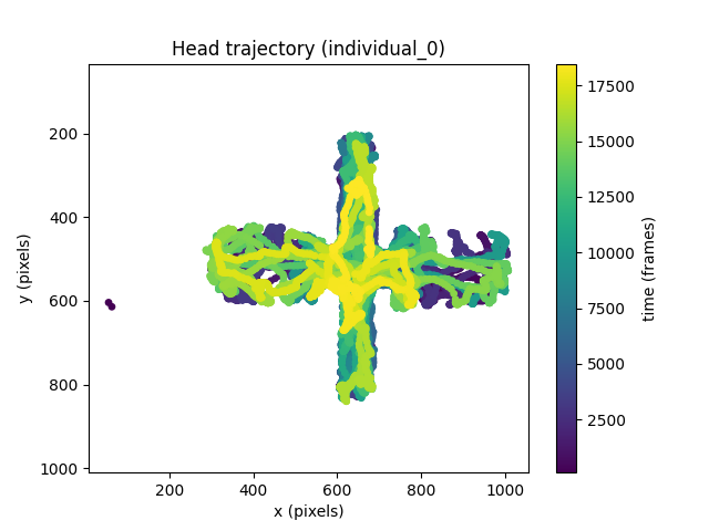
We can see that the majority of the head trajectory data is within a cruciform shape. This is because the dataset is of a mouse moving on an Elevated Plus Maze. We can actually verify this is the case by overlaying the head trajectory on the sample frame of the dataset.

# read sample frame
frame_path = sample_data.fetch_dataset_paths(
    "SLEAP_single-mouse_EPM.analysis.h5"
)["frame"]
im = plt.imread(frame_path)


# plot sample frame
fig, ax = plt.subplots(1, 1)
ax.imshow(im)

# plot head trajectory with semi-transparent markers
sc = ax.scatter(
    midpoint_ears.sel(individuals=mouse_name, space="x"),
    midpoint_ears.sel(individuals=mouse_name, space="y"),
    s=15,
    c=midpoint_ears.time,
    cmap="viridis",
    marker="o",
    alpha=0.05,  # transparency
)

ax.axis("equal")
ax.set_xlabel("x (pixels)")
ax.set_ylabel("y (pixels)")
# No need to invert the y-axis now, since the image is plotted
# using a pixel coordinate system with origin on the top left of the image
ax.set_title(f"Head trajectory ({mouse_name})")

fig.show()

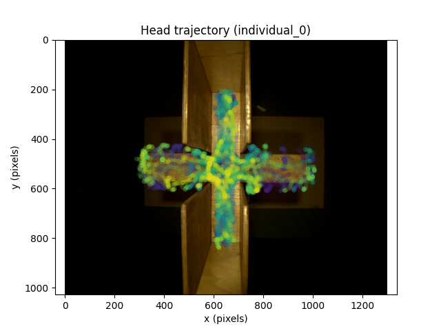
The overlaid plot suggests the mouse spends most of its time in the covered arms of the maze.

Visualise the head vector

To visually check our computation of the head vector, it is easier to select a subset of the data. We can focus on the trajectory of the head when the mouse is within a small rectangular area and time window.

# area of interest
xmin, ymin = 600, 665  # pixels
x_delta, y_delta = 125, 100  # pixels

# time window
time_window = range(1650, 1671)  # frames

For that subset of the data, we now plot the head vector.

fig, ax = plt.subplots(1, 1)
mouse_name = ds.individuals.values[0]

# plot midpoint between the ears, and color based on time
sc = ax.scatter(
    midpoint_ears.sel(individuals=mouse_name, space="x", time=time_window),
    midpoint_ears.sel(individuals=mouse_name, space="y", time=time_window),
    s=50,
    c=midpoint_ears.time[time_window],
    cmap="viridis",
    marker="*",
)

# plot snout, and color based on time
sc = ax.scatter(
    position.sel(
        individuals=mouse_name, space="x", time=time_window, keypoints="snout"
    ),
    position.sel(
        individuals=mouse_name, space="y", time=time_window, keypoints="snout"
    ),
    s=50,
    c=position.time[time_window],
    cmap="viridis",
    marker="o",
)

# plot the computed head vector
ax.quiver(
    midpoint_ears.sel(individuals=mouse_name, space="x", time=time_window),
    midpoint_ears.sel(individuals=mouse_name, space="y", time=time_window),
    head_vector.sel(individuals=mouse_name, space="x", time=time_window),
    head_vector.sel(individuals=mouse_name, space="y", time=time_window),
    angles="xy",
    scale=1,
    scale_units="xy",
    headwidth=7,
    headlength=9,
    headaxislength=9,
    color="gray",
)

ax.axis("equal")
ax.set_xlim(xmin, xmin + x_delta)
ax.set_ylim(ymin, ymin + y_delta)
ax.set_xlabel("x (pixels)")
ax.set_ylabel("y (pixels)")
ax.set_title(f"Zoomed in head vector ({mouse_name})")
ax.invert_yaxis()
fig.colorbar(
    sc,
    ax=ax,
    label=f"time ({ds.attrs['time_unit']})",
    ticks=list(time_window)[0::2],
)

ax.legend(
    [
        "midpoint_ears",
        "snout",
        "head_vector",
    ],
    loc="best",
)

fig.show()

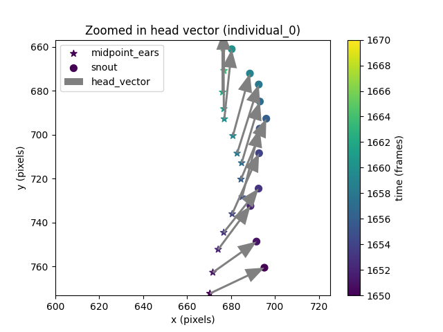
From the plot we can confirm the head vector goes from the midpoint between the ears to the snout, as we defined it.

Express the head vector in polar coordinates

A convenient way to inspect the orientation of a vector in 2D is by expressing it in polar coordinates. We can do this with the vector function cart2pol:

head_vector_polar = cart2pol(head_vector)

print(head_vector_polar)

<xarray.DataArray 'position' (time: 18485, space_pol: 2, individuals: 1)> Size: 148kB
nan nan nan nan nan nan nan nan ... 1.247 18.14 1.126 20.92 1.19 15.59 1.28
Coordinates:
  * time         (time) int64 148kB 0 1 2 3 4 ... 18480 18481 18482 18483 18484
  * individuals  (individuals) <U12 48B 'individual_0'
  * space_pol    (space_pol) <U3 24B 'rho' 'phi'

Notice how the resulting array has a space_pol dimension with two coordinates: rho and phi. These are the polar coordinates of the head vector.

The coordinate rho is the norm (i.e., magnitude, length) of the vector. In our case, the distance from the midpoint between the ears to the snout. The coordinate phi is the orientation of the head vector relative to the positive x-axis, and ranges from -pi to pi (following the atan2 convention).

In our coordinate system, phi will be positive if the shortest path from the positive x-axis to the vector is clockwise. Conversely, phi will be negative if the shortest path from the positive x-axis to the vector is anti-clockwise.

Histogram of rho values

Since rho is the distance between the ears’ midpoint and the snout, we would expect rho to be approximately constant in this data. We can check this by plotting a histogram of its values across the whole clip.

fig, ax = plt.subplots(1, 1)

# plot histogram using xarray's built-in histogram function
rho_data = head_vector_polar.sel(individuals=mouse_name, space_pol="rho")
rho_data.plot.hist(bins=50, ax=ax, edgecolor="lightgray", linewidth=0.5)

# add mean
ax.axvline(
    x=rho_data.mean().values,
    c="b",
    linestyle="--",
)


# add median
ax.axvline(
    x=rho_data.median().values,
    c="r",
    linestyle="-",
)

# add legend
ax.legend(
    [
        f"mean = {np.nanmean(rho_data):.2f} pixels",
        f"median = {np.nanmedian(rho_data):.2f} pixels",
    ],
    loc="best",
)
ax.set_ylabel("count")
ax.set_xlabel("rho (pixels)")
fig.show()

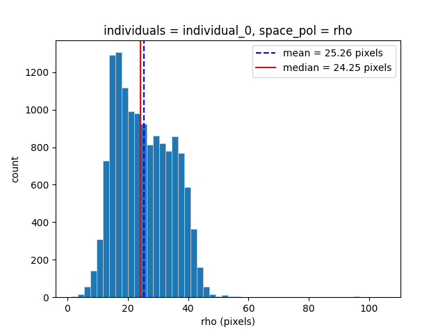
We can see that there is some spread in the value of rho in this dataset. This may be due to noise in the detection of the head keypoints, or due to the mouse tipping its snout upwards during the recording.

Histogram of phi values

We can also explore which phi values are most common in the dataset with a circular histogram.

# compute number of bins
bin_width_deg = 5  # width of the bins in degrees
n_bins = int(360 / bin_width_deg)

# initialise figure with polar projection
fig = plt.figure()
ax = fig.add_subplot(projection="polar")

# plot histogram using xarray's built-in histogram function
head_vector_polar.sel(individuals=mouse_name, space_pol="phi").plot.hist(
    bins=np.linspace(-np.pi, np.pi, n_bins + 1), ax=ax
)

# axes settings
ax.set_title("phi histogram")
ax.set_theta_direction(-1)  # theta increases in clockwise direction
ax.set_theta_offset(0)  # set zero at the right
ax.set_xlabel("")  # remove default x-label from xarray's plot.hist()

# set xticks to match the phi values in degrees
n_xtick_edges = 9
ax.set_xticks(np.linspace(0, 2 * np.pi, n_xtick_edges)[:-1])
xticks_in_deg = (
    list(range(0, 180 + 45, 45)) + list(range(0, -180, -45))[-1:0:-1]
)
ax.set_xticklabels([str(t) + "\N{DEGREE SIGN}" for t in xticks_in_deg])

fig.show()

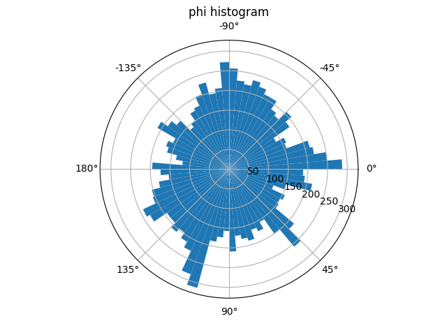
The phi circular histogram shows that the head vector appears at a variety of orientations in this dataset.

Polar plot of the head vector within a time window

We can also use a polar plot to represent the head vector in time. This way we can visualise the head vector in a coordinate system that translates with the mouse but is always parallel to the pixel coordinate system. Again, this will be easier to visualise if we focus on a small time window.

# select phi values within a time window
phi = head_vector_polar.sel(
    individuals=mouse_name,
    space_pol="phi",
    time=time_window,
).values

# plot tip of the head vector within that window, and color based on time
fig = plt.figure()
ax = fig.add_subplot(projection="polar")
sc = ax.scatter(
    phi,
    np.ones_like(phi),  # assign a constant value rho=1 for visualization
    c=time_window,
    cmap="viridis",
    s=50,
)

# axes settings
ax.set_theta_direction(-1)  # theta increases in clockwise direction
ax.set_theta_offset(0)  # set zero at the right
cax = fig.colorbar(
    sc,
    ax=ax,
    label=f"time ({ds.attrs['time_unit']})",
    ticks=list(time_window)[0::2],
)

# set xticks to match the phi values in degrees
n_xtick_edges = 9
ax.set_xticks(np.linspace(0, 2 * np.pi, n_xtick_edges)[:-1])
xticks_in_deg = (
    list(range(0, 180 + 45, 45)) + list(range(0, -180, -45))[-1:0:-1]
)
ax.set_xticklabels([str(t) + "\N{DEGREE SIGN}" for t in xticks_in_deg])

fig.show()

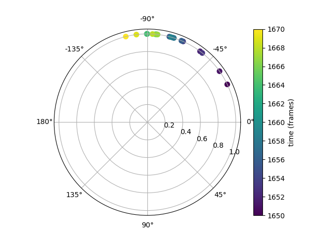
In the polar plot above, the midpoint between the ears is at the centre of the plot. The tip of the head vector (the snout) is represented with color markers at a constant rho value of 1. Markers are colored by frame. The polar plot shows how in this small time window of 20 frames, the head of the mouse turned anti-clockwise.

Convert polar coordinates to cartesian

movement also provides a pol2cart convenience function to transform a vector in polar coordinates back to cartesian.

head_vector_cart = pol2cart(head_vector_polar)

print(head_vector_cart)

<xarray.DataArray 'position' (time: 18485, space: 2, individuals: 1)> Size: 148kB
nan nan nan nan nan nan nan nan ... 17.93 7.802 16.38 7.777 19.42 4.465 14.94
Coordinates:
  * time         (time) int64 148kB 0 1 2 3 4 ... 18480 18481 18482 18483 18484
  * individuals  (individuals) <U12 48B 'individual_0'
  * space        (space) <U1 8B 'x' 'y'

Note that the resulting head_vector_cart array has a space dimension with two coordinates: x and y.