
Note
Go to the end to download the full example code. or to run this example in your browser via Binder
Smooth pose tracks#
Smooth pose tracks using the rolling median and Savitzky-Golay filters.
Imports#
import matplotlib.pyplot as plt
from scipy.signal import welch

from movement import sample_data
from movement.filtering import (
    interpolate_over_time,
    rolling_filter,
    savgol_filter,
)
Load a sample dataset#
Let’s load a sample dataset and print it to inspect its contents.
Note that if you are running this notebook interactively, you can simply
type the variable name (here ds_wasp) in a cell to get an interactive
display of the dataset’s contents.
ds_wasp = sample_data.fetch_dataset("DLC_single-wasp.predictions.h5")
print(ds_wasp)
<xarray.Dataset> Size: 61kB
Dimensions:      (time: 1085, space: 2, keypoints: 2, individuals: 1)
Coordinates:
  * time         (time) float64 9kB 0.0 0.025 0.05 0.075 ... 27.05 27.07 27.1
  * space        (space) <U1 8B 'x' 'y'
  * keypoints    (keypoints) <U7 56B 'head' 'stinger'
  * individuals  (individuals) <U12 48B 'individual_0'
Data variables:
    position     (time, space, keypoints, individuals) float64 35kB 1.086e+03...
    confidence   (time, keypoints, individuals) float64 17kB 0.05305 ... 0.0
Attributes:
    source_software:  DeepLabCut
    ds_type:          poses
    fps:              40.0
    time_unit:        seconds
    source_file:      /home/runner/.movement/data/poses/DLC_single-wasp.predi...
    frame_path:       /home/runner/.movement/data/frames/single-wasp_frame-10...
We see that the dataset contains the 2D pose tracks and confidence scores for a single wasp, generated with DeepLabCut. The wasp is tracked at two keypoints: “head” and “stinger” in a video that was recorded at 40 fps and lasts for approximately 27 seconds.
Define a plotting function#
Let’s define a plotting function to help us visualise the effects of
smoothing both in the time and frequency domains.
The function takes as inputs two datasets containing raw and smooth data
respectively, and plots the position time series and power spectral density
(PSD) for a given individual and keypoint. The function also allows you to
specify the spatial coordinate (x or y) and a time range to focus on.
def plot_raw_and_smooth_timeseries_and_psd(
    ds_raw,
    ds_smooth,
    individual=None,
    keypoint="stinger",
    space="x",
    time_range=None,
):
    # If no individual is specified, use the first one
    if individual is None:
        individual = ds_raw.individuals[0]
    # If no time range is specified, plot the entire time series
    if time_range is None:
        time_range = slice(0, ds_raw.time[-1])

    selection = {
        "time": time_range,
        "individuals": individual,
        "keypoints": keypoint,
        "space": space,
    }

    fig, ax = plt.subplots(2, 1, figsize=(10, 6))

    for ds, color, label in zip(
        [ds_raw, ds_smooth], ["k", "r"], ["raw", "smooth"], strict=False
    ):
        # plot position time series
        pos = ds.position.sel(**selection)
        ax[0].plot(
            pos.time,
            pos,
            color=color,
            lw=2,
            alpha=0.7,
            label=f"{label} {space}",
        )

        # interpolate data to remove NaNs in the PSD calculation
        pos_interp = interpolate_over_time(pos, fill_value="extrapolate")

        # compute and plot the PSD
        freq, psd = welch(pos_interp, fs=ds.fps, nperseg=256)
        ax[1].semilogy(
            freq,
            psd,
            color=color,
            lw=2,
            alpha=0.7,
            label=f"{label} {space}",
        )

    ax[0].set_ylabel(f"{space} position (px)")
    ax[0].set_xlabel("Time (s)")
    ax[0].set_title("Time Domain")
    ax[0].legend()

    ax[1].set_ylabel("PSD (px$^2$/Hz)")
    ax[1].set_xlabel("Frequency (Hz)")
    ax[1].set_title("Frequency Domain")
    ax[1].legend()

    plt.tight_layout()
    fig.show()
Smoothing with a rolling median filter#
Using the movement.filtering.rolling_filter() function on the
position data variable, we can apply a rolling median filter
over a 0.1-second window (4 frames) to the wasp dataset.
As the window parameter is defined in number of observations,
we can simply multiply the desired time window by the frame rate
of the video. We will also create a copy of the dataset to avoid
modifying the original data.
Here we use the default statistic="median" option, which is a sensible
choice for smoothing time-series data while being robust to outliers.
You can also use
rolling_filter() to compute
the rolling mean, maximum, and minimum values (instead of the median), by
setting statistic to "mean", "max", or "min", respectively.
window = int(0.1 * ds_wasp.fps)
ds_wasp_smooth = ds_wasp.copy()
ds_wasp_smooth.update(
    {
        "position": rolling_filter(
            ds_wasp.position, window, statistic="median", print_report=True
        )
    }
)
No missing points (marked as NaN) in input.
No missing points (marked as NaN) in output.
We see from the printed report that the dataset has no missing values neither before nor after smoothing. Let’s visualise the effects of applying the rolling median filter in the time and frequency domains.
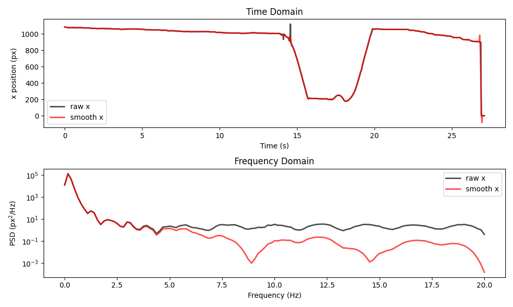
plot_raw_and_smooth_timeseries_and_psd(
    ds_wasp, ds_wasp_smooth, keypoint="stinger"
)
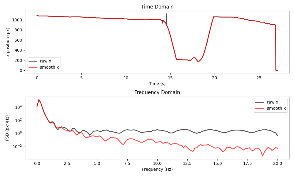
We see that applying the filter has removed the “spikes” present around the 14 second mark in the raw data. However, it has not dealt with the big shift occurring during the final second. In the frequency domain, we can see that the filter has reduced the power in the high-frequency components, without affecting the low frequency components.
This shows what the rolling median is good for: removing brief “spikes” (e.g. a keypoint abruptly jumping to a different location for a frame or two) and high-frequency “jitter” (often present due to pose estimation working on a per-frame basis).
Choosing parameters for the rolling filter#
We can control the behaviour of the rolling filter
via three parameters: window, min_periods and statistic which was
mentioned above.
To better understand the effect of these parameters, let’s use a
dataset that contains missing values.
ds_mouse = sample_data.fetch_dataset("SLEAP_single-mouse_EPM.analysis.h5")
print(ds_mouse)
<xarray.Dataset> Size: 1MB
Dimensions:      (time: 18485, space: 2, keypoints: 6, individuals: 1)
Coordinates:
  * time         (time) float64 148kB 0.0 0.03333 0.06667 ... 616.1 616.1 616.1
  * space        (space) <U1 8B 'x' 'y'
  * keypoints    (keypoints) <U9 216B 'snout' 'left_ear' ... 'tail_end'
  * individuals  (individuals) <U4 16B 'id_0'
Data variables:
    position     (time, space, keypoints, individuals) float32 887kB nan ... ...
    confidence   (time, keypoints, individuals) float32 444kB nan nan ... 0.7607
Attributes:
    source_software:  SLEAP
    ds_type:          poses
    fps:              30.0
    time_unit:        seconds
    source_file:      /home/runner/.movement/data/poses/SLEAP_single-mouse_EP...
    frame_path:       /home/runner/.movement/data/frames/single-mouse_EPM_fra...
The dataset contains a single mouse with six keypoints tracked in 2D space. The video was recorded at 30 fps and lasts for ~616 seconds. We can see that there are some missing values, indicated as “nan” in the printed dataset. Let’s apply the rolling median filter over a 0.1-second window (3 frames) to the dataset.
window = int(0.1 * ds_mouse.fps)
ds_mouse_smooth = ds_mouse.copy()
ds_mouse_smooth.update(
    {
        "position": rolling_filter(
            ds_mouse.position, window, statistic="median", print_report=True
        )
    }
)
Missing points (marked as NaN) in input:

keypoints                  snout           left_ear          right_ear             centre          tail_base            tail_end
individuals
id_0         4494/18485 (24.31%)  513/18485 (2.78%)  533/18485 (2.88%)  490/18485 (2.65%)  704/18485 (3.81%)  2496/18485 (13.5%)
Missing points (marked as NaN) in output:

keypoints                  snout           left_ear          right_ear             centre          tail_base             tail_end
individuals
id_0         5106/18485 (27.62%)  678/18485 (3.67%)  695/18485 (3.76%)  640/18485 (3.46%)  913/18485 (4.94%)  3103/18485 (16.79%)
The report informs us that the raw data contains NaN values, most of which
occur at the snout and tail_end keypoints. After filtering, the
number of NaNs has increased. This is because the default behaviour of the
rolling filter is to propagate NaN values, i.e. if any value in the rolling
window is NaN, the output will also be NaN.
To modify this behaviour, you can set the value of the min_periods
parameter to an integer value. This parameter determines the minimum number
of non-NaN values required in the window for the output to be non-NaN.
For example, setting min_periods=2 means that two non-NaN values in the
window are sufficient for the median to be calculated. Let’s try this.
ds_mouse_smooth.update(
    {
        "position": rolling_filter(
            ds_mouse.position,
            window,
            min_periods=2,
            statistic="median",
            print_report=True,
        )
    }
)
Missing points (marked as NaN) in input:

keypoints                  snout           left_ear          right_ear             centre          tail_base            tail_end
individuals
id_0         4494/18485 (24.31%)  513/18485 (2.78%)  533/18485 (2.88%)  490/18485 (2.65%)  704/18485 (3.81%)  2496/18485 (13.5%)
Missing points (marked as NaN) in output:

keypoints                 snout           left_ear          right_ear             centre          tail_base             tail_end
individuals
id_0         4455/18485 (24.1%)  487/18485 (2.63%)  507/18485 (2.74%)  465/18485 (2.52%)  673/18485 (3.64%)  2428/18485 (13.13%)
We see that this time the number of NaN values has decreased
across all keypoints.
Let’s visualise the effects of the rolling median filter in the time and
frequency domains. Here we focus on the first 80 seconds for the snout
keypoint. You can adjust the keypoint and time_range arguments to
explore other parts of the data.
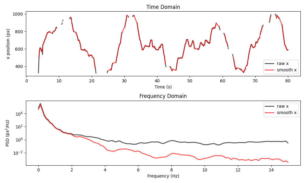
plot_raw_and_smooth_timeseries_and_psd(
    ds_mouse, ds_mouse_smooth, keypoint="snout", time_range=slice(0, 80)
)
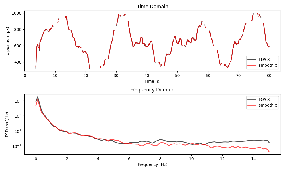
The smoothing once again reduces the power of high-frequency components, but the resulting time series stays quite close to the raw data.
What happens if we increase the window to 2 seconds (60 frames)?
window = int(2 * ds_mouse.fps)
ds_mouse_smooth.update(
    {
        "position": rolling_filter(
            ds_mouse.position,
            window,
            min_periods=2,
            statistic="median",
            print_report=True,
        )
    }
)
Missing points (marked as NaN) in input:

keypoints                  snout           left_ear          right_ear             centre          tail_base            tail_end
individuals
id_0         4494/18485 (24.31%)  513/18485 (2.78%)  533/18485 (2.88%)  490/18485 (2.65%)  704/18485 (3.81%)  2496/18485 (13.5%)
Missing points (marked as NaN) in output:

keypoints               snout          left_ear         right_ear            centre         tail_base           tail_end
individuals
id_0         795/18485 (4.3%)  80/18485 (0.43%)  80/18485 (0.43%)  80/18485 (0.43%)  80/18485 (0.43%)  239/18485 (1.29%)
The number of NaN values has decreased even further. That’s because the chance of finding at least 2 valid values within a 2-second window (i.e. 60 frames) is quite high. Let’s plot the results for the same keypoint and time range as before.
plot_raw_and_smooth_timeseries_and_psd(
    ds_mouse, ds_mouse_smooth, keypoint="snout", time_range=slice(0, 80)
)
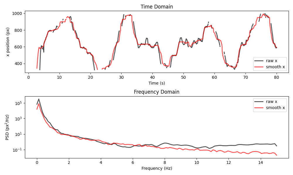
We see that the filtered time series is much smoother and it has even
“bridged” over some small gaps. That said, it often deviates from the raw
data, in ways that may not be desirable, depending on the application.
Here, our choice of window may be too large.
In general, you should choose a window that is small enough to
preserve the original data structure, but large enough to remove
“spikes” and high-frequency noise. Always inspect the results to ensure
that the filter is not removing important features.
Smoothing with a Savitzky-Golay filter#
Here we apply the movement.filtering.savgol_filter() function
(a wrapper around scipy.signal.savgol_filter()), to the position
data variable.
The Savitzky-Golay filter is a polynomial smoothing filter that can be
applied to time series data on a rolling window basis.
A polynomial with a degree specified by polyorder is applied to each
data segment defined by the size window.
The value of the polynomial at the midpoint of each window is then
used as the output value.
Let’s try it on the mouse dataset, this time using a 0.2-second
window (i.e. 6 frames) and the default polyorder=2 for smoothing.
As before, we first compute the corresponding number of observations
to be used as the window size.
window = int(0.2 * ds_mouse.fps)
ds_mouse_smooth.update(
    {"position": savgol_filter(ds_mouse.position, window, print_report=True)}
)
Missing points (marked as NaN) in input:

keypoints                  snout           left_ear          right_ear             centre          tail_base            tail_end
individuals
id_0         4494/18485 (24.31%)  513/18485 (2.78%)  533/18485 (2.88%)  490/18485 (2.65%)  704/18485 (3.81%)  2496/18485 (13.5%)
Missing points (marked as NaN) in output:

keypoints                  snout           left_ear         right_ear             centre           tail_base             tail_end
individuals
id_0         5810/18485 (31.43%)  895/18485 (4.84%)  905/18485 (4.9%)  839/18485 (4.54%)  1186/18485 (6.42%)  3801/18485 (20.56%)
We see that the number of NaN values has increased after filtering. This is
for the same reason as with the rolling filter (in its default mode), i.e.
if there is at least one NaN value in the window, the output will be NaN.
Unlike the rolling filter, the Savitzky-Golay filter does not provide a
min_periods parameter to control this behaviour. Let’s visualise the
effects in the time and frequency domains.
plot_raw_and_smooth_timeseries_and_psd(
    ds_mouse, ds_mouse_smooth, keypoint="snout", time_range=slice(0, 80)
)
Once again, the power of high-frequency components has been reduced, but more missing values have been introduced.
Now let’s apply the same Savitzky-Golay filter to the wasp dataset.
window = int(0.2 * ds_wasp.fps)
ds_wasp_smooth.update(
    {"position": savgol_filter(ds_wasp.position, window, print_report=True)}
)
No missing points (marked as NaN) in input.
No missing points (marked as NaN) in output.
plot_raw_and_smooth_timeseries_and_psd(
    ds_wasp, ds_wasp_smooth, keypoint="stinger"
)
This example shows two important limitations of the Savitzky-Golay filter.
First, the filter can introduce artefacts around sharp boundaries. For
example, focus on what happens around the sudden drop in position
during the final second. Second, the PSD appears to have large periodic
drops at certain frequencies. Both of these effects vary with the
choice of window and polyorder. You can read more about these
and other limitations of the Savitzky-Golay filter in
this paper.
Combining multiple smoothing filters#
We can also combine multiple smoothing filters by applying them
sequentially. For example, we can first apply the rolling median filter with
a small window to remove “spikes” and then apply the Savitzky-Golay
filter with a larger window to further smooth the data.
Between the two filters, we can interpolate over small gaps to avoid the
excessive proliferation of NaN values. Let’s try this on the mouse dataset.
# First, we will apply the rolling median filter.
window = int(0.1 * ds_mouse.fps)
ds_mouse_smooth.update(
    {
        "position": rolling_filter(
            ds_mouse.position, window, min_periods=2, statistic="median"
        )
    }
)

# Next, let's linearly interpolate over gaps smaller
# than 1 second (30 frames).
ds_mouse_smooth.update(
    {"position": interpolate_over_time(ds_mouse_smooth.position, max_gap=30)}
)

# Finally, let's apply the Savitzky-Golay filter
# over a 0.4-second window (12 frames).
window = int(0.4 * ds_mouse.fps)
ds_mouse_smooth.update(
    {"position": savgol_filter(ds_mouse_smooth.position, window)}
)
A record of all applied operations is stored in the log attribute of the
ds_mouse_smooth.position data array. Let’s inspect it to summarise
what we’ve done.
print(ds_mouse_smooth.position.log)
[
  {
    "operation": "rolling_filter",
    "datetime": "2025-09-19 14:26:59.944754",
    "window": "3",
    "statistic": "'median'",
    "min_periods": "2",
    "print_report": "False"
  },
  {
    "operation": "interpolate_over_time",
    "datetime": "2025-09-19 14:26:59.970506",
    "method": "'linear'",
    "max_gap": "30",
    "print_report": "False"
  },
  {
    "operation": "savgol_filter",
    "datetime": "2025-09-19 14:26:59.974389",
    "window": "12",
    "polyorder": "2",
    "print_report": "False"
  }
]
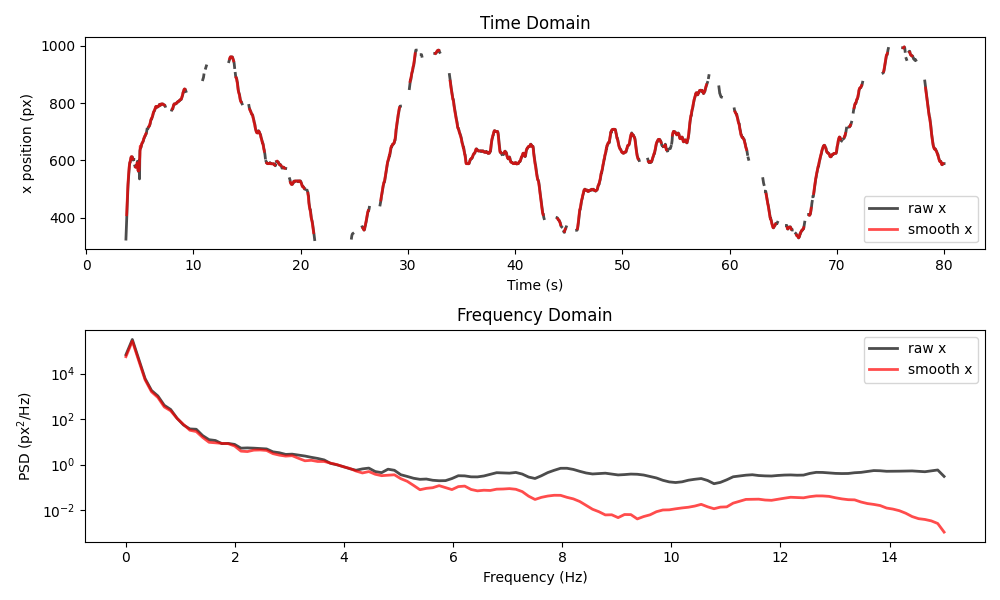
Now let’s visualise the difference between the raw data and the final smoothed result.
plot_raw_and_smooth_timeseries_and_psd(
    ds_mouse,
    ds_mouse_smooth,
    keypoint="snout",
    time_range=slice(0, 80),
)
Feel free to play around with the parameters of the applied filters and to also look at other keypoints and time ranges.
See also
Filtering multiple data variables in the Drop outliers and interpolate example.
Total running time of the script: (0 minutes 1.599 seconds)