Compute head direction

Compute the head direction vector and angle using different methods.

Imports

# For interactive plots: install ipympl with `pip install ipympl` and uncomment
# the following line in your notebook
# %matplotlib widget
import numpy as np
from matplotlib import pyplot as plt

from movement import sample_data
from movement.kinematics import (
    compute_forward_vector,
    compute_forward_vector_angle,
)
from movement.plots import plot_centroid_trajectory
from movement.utils.vector import cart2pol, pol2cart

Load sample dataset

In this tutorial, we will use a sample dataset with a single individual (a mouse) and six keypoints.

ds = sample_data.fetch_dataset("DLC_single-mouse_EPM.predictions.h5")

print(ds)
print("-----------------------------")
print(f"Individuals: {ds.individuals.values}")
print(f"Keypoints: {ds.keypoints.values}")

<xarray.Dataset> Size: 4MB
Dimensions:      (time: 18485, space: 2, keypoints: 8, individuals: 1)
Coordinates:
  * time         (time) float64 148kB 0.0 0.03333 0.06667 ... 616.1 616.1 616.1
  * space        (space) <U1 8B 'x' 'y'
  * keypoints    (keypoints) <U13 416B 'snout' 'left_ear' ... 'tail_end'
  * individuals  (individuals) <U12 48B 'individual_0'
Data variables:
    position     (time, space, keypoints, individuals) float64 2MB 508.4 ... ...
    confidence   (time, keypoints, individuals) float64 1MB 0.0002829 ... 0.9978
Attributes:
    source_software:  DeepLabCut
    ds_type:          poses
    fps:              30.0
    time_unit:        seconds
    source_file:      /home/runner/.movement/data/poses/DLC_single-mouse_EPM....
    frame_path:       /home/runner/.movement/data/frames/single-mouse_EPM_fra...
-----------------------------
Individuals: ['individual_0']
Keypoints: ['snout' 'left_ear' 'right_ear' 'centre' 'lateral_left' 'lateral_right'
 'tailbase' 'tail_end']

The loaded dataset ds contains two data arrays:position and confidence. In this tutorial, we will only use the position data array. We use the squeeze() method to remove the redundant individuals dimension, as there is only one individual in this dataset.

position = ds.position.squeeze()

Visualise the head trajectory

We can start by visualising the head trajectory, taking the midpoint between the ears as an estimate for the head centre. We will overlay that on a single video frame that comes as part of the sample dataset.

The plot_centroid_trajectory() function can help you visualise the trajectory of any keypoint in the data. Passing a list of keypoints, in this case ["left_ear", "right_ear"], will plot the centroid (midpoint) of the selected keypoints. By default, the first individual in the dataset is shown.

# Create figure and axis
fig, ax = plt.subplots(1, 1)

# Plot a single frame from the dataset (its path is stored as an attribute)
frame = plt.imread(ds.frame_path)
ax.imshow(frame)

# Plot the trajectory of the head centre
plot_centroid_trajectory(
    ds.position,
    keypoints=["left_ear", "right_ear"],
    ax=ax,
    # arguments forwarded to plt.scatter
    s=10,
    cmap="viridis",
    marker="o",
    alpha=0.05,
)

# Adjust title
ax.set_title("Head trajectory")
ax.set_ylim(frame.shape[0], 0)  # match y-axis limits to image coordinates
ax.set_xlabel("x (pixels)")
ax.set_ylabel("y (pixels)")
ax.collections[0].colorbar.set_label("Time (seconds)")
fig.show()

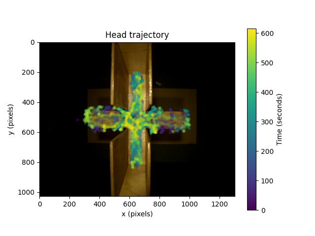
We can see that most of the head trajectory data is within a cruciform shape, because the mouse is moving on an Elevated Plus Maze. The plot suggests the mouse spends most of its time in the covered arms of the maze (the vertical arms).

Compute the head-to-snout vector

We can define the head direction as the vector from the midpoint between the ears to the snout.

# Compute the head centre as the midpoint between the ears
midpoint_ears = position.sel(keypoints=["left_ear", "right_ear"]).mean(
    dim="keypoints"
)
# Snout position
# (`drop=True` removes the keypoints dimension, which is now redundant)
snout = position.sel(keypoints="snout", drop=True)

# Compute the head vector as the difference vector between the snout position
# and the head-centre position.
head_to_snout = snout - midpoint_ears

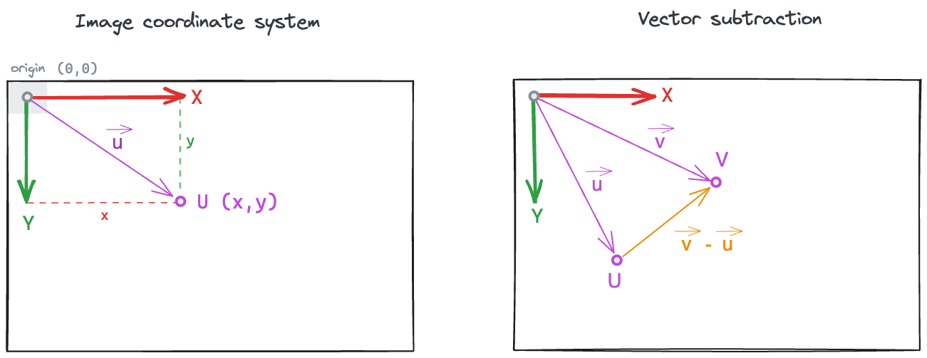
Vector subtraction

Note that any position data point can be seen as a point \(U\) in the 2D plane, or as a 2D vector \(\vec{u}\) that goes from the image coordinate system origin (by default, the centre of the top-left pixel) to the point \(U\) (see left subplot).

The vector that goes from point \(U\) to point \(V\) can be computed as the difference \(\vec{v} - \vec{u}\) (see right subplot).

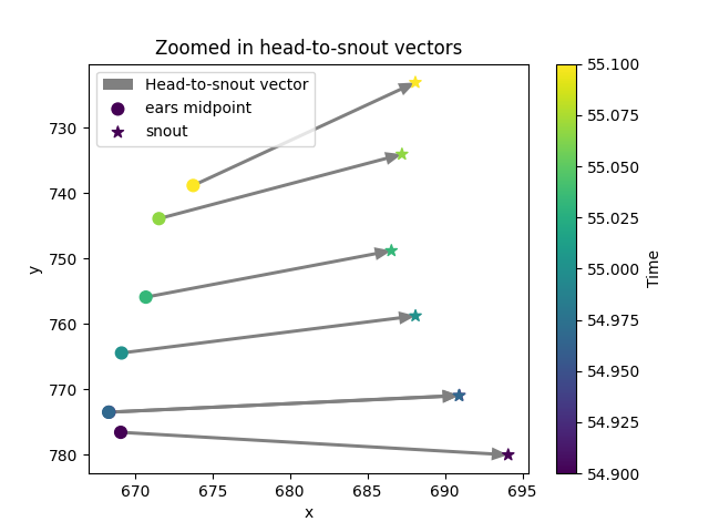
Let’s validate our computation by plotting the head-to-snout vector alongside the midpoint between the ears and the snout position. We will do this for a small time window to make the plot more readable.

# Time window to restrict the plot
time_window = slice(54.9, 55.1)  # seconds

fig, ax = plt.subplots()

# Plot the computed head-to-snout vector originating from the ears midpoint
ax.quiver(
    midpoint_ears.sel(space="x", time=time_window),
    midpoint_ears.sel(space="y", time=time_window),
    head_to_snout.sel(space="x", time=time_window),
    head_to_snout.sel(space="y", time=time_window),
    color="gray",
    angles="xy",
    scale=1,
    scale_units="xy",
    headwidth=4,
    headlength=5,
    headaxislength=5,
    label="Head-to-snout vector",
)

# Plot midpoint between the ears within the time window
plot_centroid_trajectory(
    midpoint_ears.sel(time=time_window),
    ax=ax,
    s=60,
    label="ears midpoint",
)

# Plot the snout position within the time window
plot_centroid_trajectory(
    snout.sel(time=time_window),
    ax=ax,
    s=60,
    marker="*",
    label="snout",
)

# Calling plot_centroid_trajectory twice will add 2 identical colorbars
# so we remove 1
ax.collections[2].colorbar.remove()

ax.set_title("Zoomed in head-to-snout vectors")
ax.invert_yaxis()  # invert y-axis to match image coordinates
ax.legend(loc="upper left")

<matplotlib.legend.Legend object at 0x7f0c3cd6e120>

Head-to-snout vector in polar coordinates

Now that we have the head-to-snout vector, we can compute its angle in 2D space. A convenient way to achieve that is to convert the vector from cartesian to polar coordinates using the cart2pol() function.

head_to_snout_polar = cart2pol(head_to_snout)

print(head_to_snout_polar)

<xarray.DataArray 'position' (time: 18485, space_pol: 2)> Size: 296kB
1.637 1.995 1.624 1.99 1.67 1.994 1.681 ... 22.11 0.937 22.12 0.9768 20.81 1.011
Coordinates:
  * time         (time) float64 148kB 0.0 0.03333 0.06667 ... 616.1 616.1 616.1
    individuals  <U12 48B 'individual_0'
  * space_pol    (space_pol) <U3 24B 'rho' 'phi'

Notice how the resulting array has a space_pol dimension with two coordinates: rho and phi. These are the polar coordinates of the head vector.

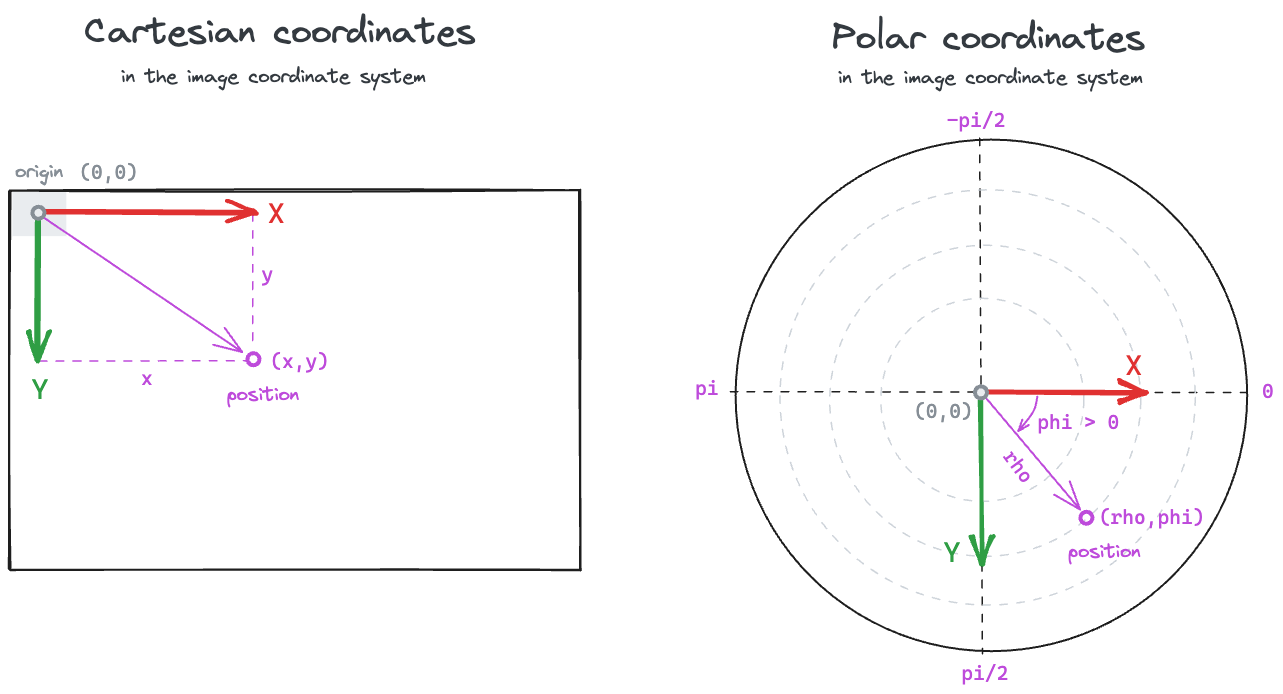
Polar coordinates

The coordinate rho is the norm (i.e., magnitude, length) of the vector. In our case, the distance from the midpoint between the ears to the snout.

The coordinate phi is the shortest angle (in radians) between the positive x-axis and the vector, and ranges from \(-\pi\) to \(\pi\) (following the atan2 convention). The phi angle is positive if the rotation from the positive x-axis to the vector is in the same direction as the rotation from the positive x-axis to the positive y-axis. In the default image coordinate system, this means phi will be positive if the rotation is clockwise, and negative if the rotation is anti-clockwise.

movement also provides a pol2cart function to transform data in polar coordinates to cartesian. Note that the resulting head_to_snout_cart array has a space dimension with two coordinates: x and y.

head_to_snout_cart = pol2cart(head_to_snout_polar)
print(head_to_snout_cart)

<xarray.DataArray 'position' (time: 18485, space: 2)> Size: 296kB
-0.6741 1.492 -0.661 1.484 -0.6864 1.522 ... 13.09 17.82 12.38 18.33 11.05 17.64
Coordinates:
  * time         (time) float64 148kB 0.0 0.03333 0.06667 ... 616.1 616.1 616.1
    individuals  <U12 48B 'individual_0'
  * space        (space) <U1 8B 'x' 'y'

Compute the “forward” vector

We can also estimate the head direction using the compute_forward_vector() function, which takes a different approach to the one we used above: it accepts a pair of bilaterally symmetric keypoints and computes the vector that originates at the midpoint between the keypoints and is perpendicular to the line connecting them.

Here we will use the two ears to find the head direction vector. We may prefer this method if we expect the snout detection to be unreliable (e.g., because it’s often occluded in a top-down camera view).

forward_vector = compute_forward_vector(
    position,
    left_keypoint="left_ear",
    right_keypoint="right_ear",
    camera_view="top_down",
)
print(forward_vector)

<xarray.DataArray 'position' (time: 18485, space: 2)> Size: 296kB
-0.01196 0.9999 -0.01182 0.9999 -0.0153 ... 0.9058 0.4111 0.9116 0.3797 0.9251
Coordinates:
  * space        (space) <U1 8B 'x' 'y'
  * time         (time) float64 148kB 0.0 0.03333 0.06667 ... 616.1 616.1 616.1
    individuals  <U12 48B 'individual_0'

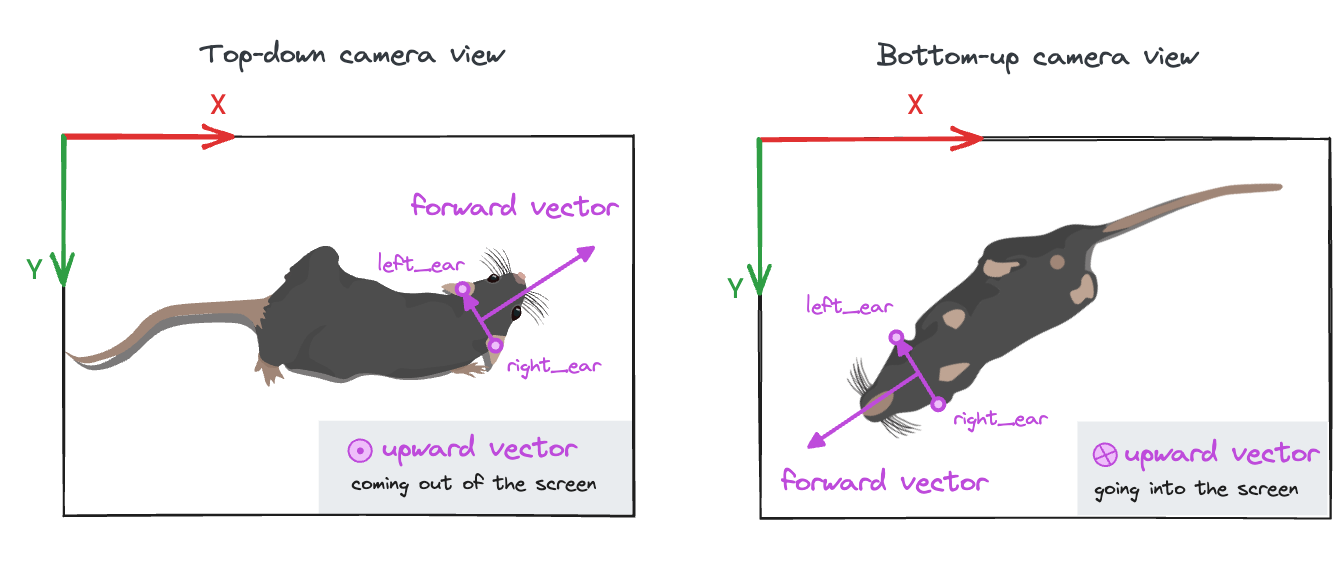
Why do we need to specify the camera view?

You can think about it in this way: in order to uniquely determine which way is forward for an animal, we need to know the orientation of the other two body axes: left-right and up-down. The left-right axis is specified by the left and right keypoints passed to the function, while we use the camera_view parameter to determine the upward direction (see image). The default view is "top_down", but it can also be "bottom_up". Other camera views are not supported at the moment.

You can use compute_forward_vector to compute the perpendicular vector to any line connecting two bilaterally symmetric keypoints. For example, you could estimate the forward direction for the pelvis given two keypoints at the hips.

Specifically for the head direction vector, you may also use the alias compute_head_direction_vector(), which makes the intent of the function clearer.

Compute head direction angle

We may want to explicitly compute the orientation of the animal’s head as an angle, rather than as a vector. We can compute this angle from the forward vector as we did with the head-to-snout vector, i.e., by converting the vector to polar coordinates and extracting the phi coordinate. However, it’s more convenient to use the compute_forward_vector_angle() function, which by default would return the same phi angle.

forward_vector_angle = compute_forward_vector_angle(
    position,
    left_keypoint="left_ear",
    right_keypoint="right_ear",
    # Optional parameters:
    reference_vector=(1, 0),  # positive x-axis
    camera_view="top_down",
    in_degrees=False,  # set to True for degrees
)
print(forward_vector_angle)

<xarray.DataArray (time: 18485)> Size: 148kB
1.583 1.583 1.586 1.588 1.585 1.585 ... 1.088 1.171 1.258 1.133 1.147 1.181
Coordinates:
  * time         (time) float64 148kB 0.0 0.03333 0.06667 ... 616.1 616.1 616.1
    individuals  <U12 48B 'individual_0'

The resulting forward_vector_angle array contains the head direction angle in radians, with respect to the positive x-axis. This means that the angle is zero when the head vector is pointing to the right of the frame. We could have also used an alternative reference vector, such as the negative y-axis (pointing to the top edge of the frame) by setting reference_vector=(0, -1).

Visualise head direction angles

We can compare the head direction angles computed from the two methods, i.e. the polar angle phi of the head-to-snout vector and the polar angle of the forward vector, by plotting their histograms in polar coordinates. First, let’s define a custom plotting function that will help us with this.

def plot_polar_histogram(da, bin_width_deg=15, ax=None):
    """Plot a polar histogram of the data in the given DataArray.

    Parameters
    ----------
    da : xarray.DataArray
        A DataArray containing angle data in radians.
    bin_width_deg : int, optional
        Width of the bins in degrees.
    ax : matplotlib.axes.Axes, optional
        The axes on which to plot the histogram.

    """
    n_bins = int(360 / bin_width_deg)

    if ax is None:
        fig, ax = plt.subplots(  # initialise figure with polar projection
            1, 1, figsize=(5, 5), subplot_kw={"projection": "polar"}
        )
    else:
        fig = ax.figure  # or use the provided axes

    # plot histogram using xarray's built-in histogram function
    da.plot.hist(
        bins=np.linspace(-np.pi, np.pi, n_bins + 1), ax=ax, density=True
    )

    # axes settings
    ax.set_theta_direction(-1)  # theta increases in clockwise direction
    ax.set_theta_offset(0)  # set zero at the right
    ax.set_xlabel("")  # remove default x-label from xarray's plot.hist()

    # set xticks to match the phi values in degrees
    n_xtick_edges = 9
    ax.set_xticks(np.linspace(0, 2 * np.pi, n_xtick_edges)[:-1])
    xticks_in_deg = (
        list(range(0, 180 + 45, 45)) + list(range(0, -180, -45))[-1:0:-1]
    )
    ax.set_xticklabels([str(t) + "\N{DEGREE SIGN}" for t in xticks_in_deg])

    return fig, ax

Now we can visualise the polar phi angles of the head_to_snout_polar array alongside the values of the forward_vector_angle array.

head_to_snout_angle = head_to_snout_polar.sel(space_pol="phi")
angle_arrays = [head_to_snout_angle, forward_vector_angle]
angle_titles = ["Head-to-snout", "Forward"]

fig, axes = plt.subplots(
    1, 2, figsize=(10, 5), subplot_kw={"projection": "polar"}
)
for i, angles in enumerate(angle_arrays):
    title = angle_titles[i]
    ax = axes[i]
    plot_polar_histogram(angles, bin_width_deg=10, ax=ax)
    ax.set_ylim(0, 0.25)  # force same y-scale (density) for both plots
    ax.set_title(title, pad=25)

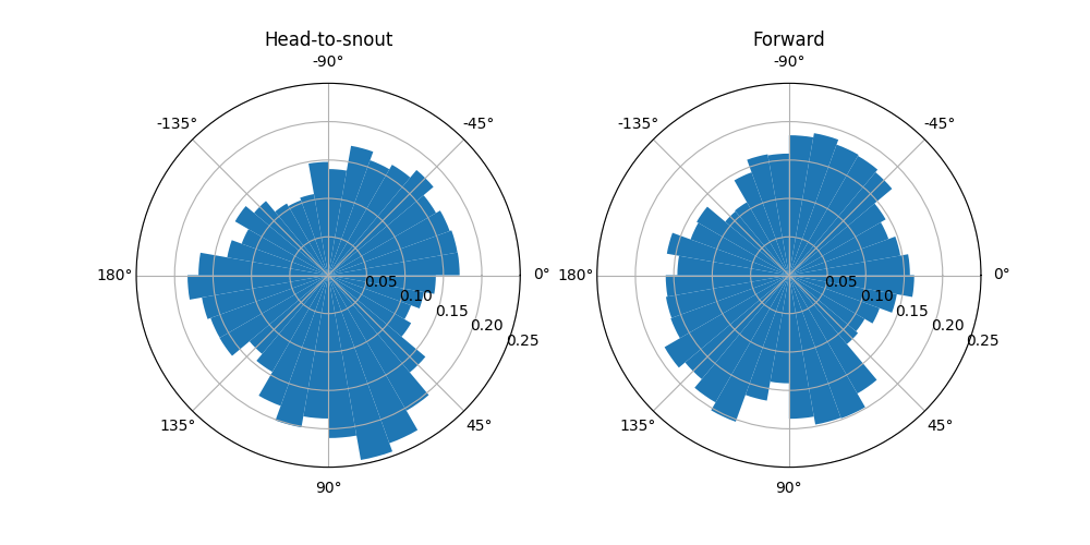
We see that the angle histograms are not identical, i.e. the two methods of computing head angle do not always yield the same results. How large are the differences between the two methods? We could check that by plotting a histogram of the differences.

angles_diff = forward_vector_angle - head_to_snout_angle
fig, ax = plot_polar_histogram(angles_diff, bin_width_deg=10)
ax.set_title("Forward vector angle - head-to-snout angle", pad=25)

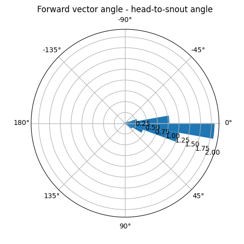
Text(0.5, 1.0, 'Forward vector angle - head-to-snout angle')

For the majority of the time, the two methods differ less than 20 degrees (2 histogram bins).