Load and visualise FreeMoCap 3D data

Load the .csv files from FreeMoCap into movement and visualise them in 3D.

Imports

To run this example, you will need to install the networkx package. You can do this by running pip install networkx in your active virtual environment (see NetworkX’s documentation for more details).

import matplotlib.pyplot as plt
import networkx as nx
import numpy as np
import pandas as pd
import xarray as xr
from mpl_toolkits.mplot3d.art3d import Line3DCollection

from movement import sample_data
from movement.io import load_poses
from movement.kinematics import compute_speed

Load sample dataset

In this tutorial we demonstrate how to import 3D data collected with FreeMoCap into movement.

FreeMoCap organises the collected data into timestamped session directories. Each session directory typically holds multiple recording subdirectories, each containing an output_data subdirectory. It is in this output_data subdirectory where FreeMoCap saves the .csv files after each recording. Each file is named after the model used to produce the data (e.g. face, body, left_hand, right_hand). Each .csv file has 3N columns, with N being the number of keypoints used by the relevant model and 3 being the number of spatial dimensions (x, y, z).

Here, we show how to load all output .csv files from a single FreeMoCap recording into a unified movement dataset.

To do this, we use a sample FreeMoCap session folder with two recordings. In the first recording, a human writes the word “hello” in the air with their index finger (recording_15_37_37_gmt+1). In the second recording, they write the word “world” (recording_15_45_49_gmt+1).

Let’s first fetch the dataset using the sample_data module and verify the folder structure.

session_dir_path = sample_data.fetch_dataset_paths(
    "FreeMoCap_hello-world_session-folder.zip"
)["poses"]

# path to output data directory for "hello" recording
output_data_dir_hello = session_dir_path.joinpath(
    "recording_15_37_37_gmt+1/output_data"
)

# path to output data directory for "world" recording
output_data_dir_world = session_dir_path.joinpath(
    "recording_15_45_49_gmt+1/output_data"
)

print("Path to session folder: ", session_dir_path)
print(
    "Path to output data directory for 'hello' recording: ",
    output_data_dir_hello,
)
print(
    "Path to output data directory for 'world' recording: ",
    output_data_dir_world,
)

Path to session folder:  /home/runner/.movement/data/poses/FreeMoCap_hello-world_session-folder
Path to output data directory for 'hello' recording:  /home/runner/.movement/data/poses/FreeMoCap_hello-world_session-folder/recording_15_37_37_gmt+1/output_data
Path to output data directory for 'world' recording:  /home/runner/.movement/data/poses/FreeMoCap_hello-world_session-folder/recording_15_45_49_gmt+1/output_data

Read FreeMoCap output files as a single movement dataset

We use the helper function below to combine all FreeMoCap output .csv files into one movement dataset. Since there is no confidence data available in the output files, we set the confidence of all keypoints to the default NaN value. We also use the default individual name id_0.

def read_freemocap_as_ds(output_data_dir):
    """Read FreeMoCap output files as a single ``movement`` dataset.

    Parameters
    ----------
    output_data_dir : pathlib.Path
        Path to the recording's output data directory holding the relevant
        ``.csv`` files.

    Returns
    -------
    xarray.Dataset
        A ``movement`` dataset containing the data from all FreeMoCap output
        files. The ``keypoints`` dimension will have the full set of keypoints
        as coordinates. The ``individuals`` dimension will have a single
        coordinate, ``id_0``. The confidence of all keypoints is set to
        the default NaN value.

    """
    list_models = ["body", "left_hand", "right_hand", "face"]
    list_datasets = []
    for m in list_models:
        # Read .csv file as a pandas DataFrame
        data_pd = pd.read_csv(
            output_data_dir.joinpath(f"mediapipe_{m}_3d_xyz.csv")
        )

        # Get list of keypoints from the dataframe, preserving the order
        # they appear in the file.
        list_keypoints = [h[:-2] for h in data_pd.columns[::3]]

        # Format data as numpy array
        data = data_pd.to_numpy()
        data = data.reshape(
            data.shape[0], int(data.shape[1] / 3), 3
        )  # time, keypoint, space

        # Transpose to align with movement dimensions
        # and add individuals dimension at the end
        data = np.transpose(data, [0, 2, 1])[..., None]

        # Read as a movement dataset
        ds = load_poses.from_numpy(
            position_array=data,  # time, space, keypoint, individual
            keypoint_names=list_keypoints,
        )
        list_datasets.append(ds)

    # Merge all datasets along keypoint dimension
    ds_all_keypoints = xr.merge(list_datasets)
    return ds_all_keypoints

We can now use the helper function to read the files in each output directory as a movement dataset.

ds_hello = read_freemocap_as_ds(output_data_dir_hello)
ds_world = read_freemocap_as_ds(output_data_dir_world)

/home/runner/work/movement/movement/examples/load_freemocap_data.py:143: FutureWarning: In a future version of xarray the default value for join will change from join='outer' to join='exact'. This change will result in the following ValueError: cannot be aligned with join='exact' because index/labels/sizes are not equal along these coordinates (dimensions): 'keypoints' ('keypoints',) The recommendation is to set join explicitly for this case.
  ds_all_keypoints = xr.merge(list_datasets)
/home/runner/work/movement/movement/examples/load_freemocap_data.py:143: FutureWarning: In a future version of xarray the default value for compat will change from compat='no_conflicts' to compat='override'. This is likely to lead to different results when combining overlapping variables with the same name. To opt in to new defaults and get rid of these warnings now use `set_options(use_new_combine_kwarg_defaults=True) or set compat explicitly.
  ds_all_keypoints = xr.merge(list_datasets)
/home/runner/work/movement/movement/examples/load_freemocap_data.py:143: FutureWarning: In a future version of xarray the default value for compat will change from compat='no_conflicts' to compat='override'. This is likely to lead to different results when combining overlapping variables with the same name. To opt in to new defaults and get rid of these warnings now use `set_options(use_new_combine_kwarg_defaults=True) or set compat explicitly.
  ds_all_keypoints = xr.merge(list_datasets)
/home/runner/work/movement/movement/examples/load_freemocap_data.py:143: FutureWarning: In a future version of xarray the default value for join will change from join='outer' to join='exact'. This change will result in the following ValueError: cannot be aligned with join='exact' because index/labels/sizes are not equal along these coordinates (dimensions): 'keypoints' ('keypoints',) The recommendation is to set join explicitly for this case.
  ds_all_keypoints = xr.merge(list_datasets)
/home/runner/work/movement/movement/examples/load_freemocap_data.py:143: FutureWarning: In a future version of xarray the default value for compat will change from compat='no_conflicts' to compat='override'. This is likely to lead to different results when combining overlapping variables with the same name. To opt in to new defaults and get rid of these warnings now use `set_options(use_new_combine_kwarg_defaults=True) or set compat explicitly.
  ds_all_keypoints = xr.merge(list_datasets)
/home/runner/work/movement/movement/examples/load_freemocap_data.py:143: FutureWarning: In a future version of xarray the default value for compat will change from compat='no_conflicts' to compat='override'. This is likely to lead to different results when combining overlapping variables with the same name. To opt in to new defaults and get rid of these warnings now use `set_options(use_new_combine_kwarg_defaults=True) or set compat explicitly.
  ds_all_keypoints = xr.merge(list_datasets)

Note that each movement dataset holds the data for all keypoints across all models used by FreeMoCap.

print(f"Number of keypoints in 'hello' dataset: {len(ds_hello.keypoints)}")
print(f"Number of keypoints in 'world' dataset: {len(ds_world.keypoints)}")

Number of keypoints in 'hello' dataset: 553
Number of keypoints in 'world' dataset: 553

Visualise a subset of the data

We would now like to visually inspect the loaded data. For clarity, we focus on the specific time window when the motion takes place, and extract the data for the single individual we have recorded and their right_hand_0006 keypoint. This keypoint tracks the right index finger used for writing in the air. Note that at the moment, FreeMoCap can only track one individual at a time.

right_index_position_hello = ds_hello.position.sel(time=range(30, 180)).sel(
    keypoints="right_hand_0006", individuals="id_0"
)
right_index_position_world = ds_world.position.sel(time=range(150)).sel(
    keypoints="right_hand_0006", individuals="id_0"
)

We use the following helper function for plotting. This function is adapted from matplotlib’s multi-coloured line example. You don’t need to understand how this function works in detail, for now it is enough to know that we will use it to plot 3D lines with a colour determined by a scalar.

def coloured_scatter_line_3d(x, y, z, c, s, ax, **lc_kwargs):
    """Plot a 3D line and colour by a scalar.

    Parameters
    ----------
    x, y, z : array-like
        x, y, z-coordinates of the line to plot.
    c : array-like
        Scalar valuesto colour the line by.
    s : float
        Size of the markers on the line.
    ax : matplotlib.axes.Axes
        Axes to plot the line on.
    **lc_kwargs : dict
        Keyword arguments to pass to ``Line3DCollection``.

    Returns
    -------
    lc : matplotlib.collections.Line3DCollection
        The line collection.

    """
    ax.scatter(x, y, z, c=c, s=s, **lc_kwargs)

    x, y, z = (np.asarray(arr).ravel() for arr in (x, y, z))
    default_kwargs = {"capstyle": "butt"}
    default_kwargs.update(lc_kwargs)

    x_mid = np.hstack((x[:1], 0.5 * (x[1:] + x[:-1]), x[-1:]))
    y_mid = np.hstack((y[:1], 0.5 * (y[1:] + y[:-1]), y[-1:]))
    z_mid = np.hstack((z[:1], 0.5 * (z[1:] + z[:-1]), z[-1:]))

    start = np.column_stack((x_mid[:-1], y_mid[:-1], z_mid[:-1]))[:, None, :]
    mid = np.column_stack((x, y, z))[:, None, :]
    end = np.column_stack((x_mid[1:], y_mid[1:], z_mid[1:]))[:, None, :]

    segments = np.concatenate((start, mid, end), axis=1)

    lc = Line3DCollection(segments, **default_kwargs)
    lc.set_array(c)
    ax.add_collection3d(lc)

    return lc

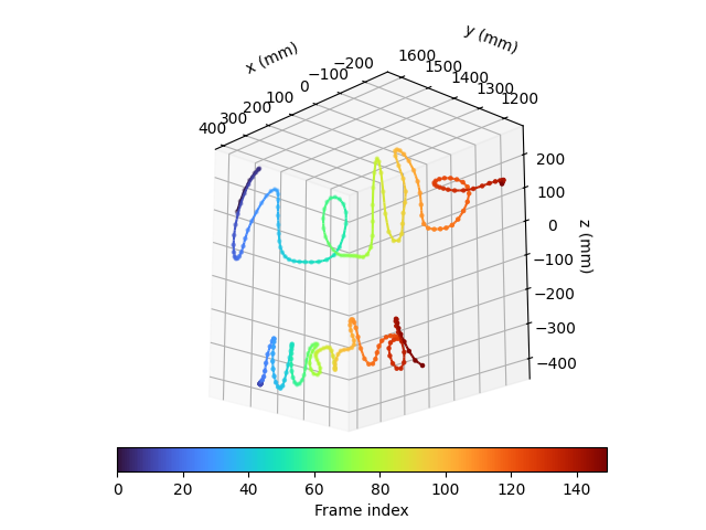
We can use the above function to plot the trajectory of the right index finger as it writes the words “hello” and “world”. We colour each point by the frame index of each recording within the time window of interest.

fig = plt.figure()
ax = fig.add_subplot(projection="3d")
colour_map = "turbo"

# plot right index finger for "hello" recording
coloured_scatter_line_3d(
    right_index_position_hello.sel(space="x"),
    right_index_position_hello.sel(space="y"),
    right_index_position_hello.sel(space="z"),
    ax=ax,
    c=right_index_position_world.time,
    s=5,
    cmap=colour_map,
)

# plot right index finger for "world" recording
# (shifted down by 400 mm in the z-axis to avoid overlap with the "hello" data)
coloured_scatter_line_3d(
    right_index_position_world.sel(space="x"),
    right_index_position_world.sel(space="y"),
    right_index_position_world.sel(space="z") - 400,
    ax=ax,
    c=right_index_position_world.time,
    s=5,
    cmap=colour_map,
)

ax.view_init(elev=-20, azim=137, roll=0)
ax.set_aspect("equal")
ax.set_xlabel("x (mm)")
ax.set_ylabel("y (mm)")
ax.set_zlabel("z (mm)")
cb = fig.colorbar(
    ax.collections[0],
    ax=ax,
    label="Frame index",
    orientation="horizontal",
    pad=-0.05,
    fraction=0.06,
)

We can also visualise how the writing speed changes along the trajectory, using the above plotting function and the movement.kinematics.compute_speed() function.

fig = plt.figure()
ax = fig.add_subplot(projection="3d")
colour_map = "inferno"

# Use movement helpers to compute speed
speed_hello = compute_speed(right_index_position_hello)
speed_world = compute_speed(right_index_position_world)

# plot right index finger for "hello" recording
coloured_scatter_line_3d(
    right_index_position_hello.sel(space="x"),
    right_index_position_hello.sel(space="y"),
    right_index_position_hello.sel(space="z"),
    ax=ax,
    c=speed_hello,
    s=5,
    cmap=colour_map,
)

# plot right index finger for "world" recording
# (shifted down by 400 mm in the z-axis to avoid overlap with the "hello" data)
coloured_scatter_line_3d(
    right_index_position_world.sel(space="x"),
    right_index_position_world.sel(space="y"),
    right_index_position_world.sel(space="z") - 400,
    ax=ax,
    c=speed_world,
    s=5,
    cmap=colour_map,
)

ax.view_init(elev=-20, azim=137, roll=0)
ax.set_aspect("equal")
ax.set_xlabel("x (mm)")
ax.set_ylabel("y (mm)")
ax.set_zlabel("z (mm)")
cb = fig.colorbar(
    ax.collections[0],
    ax=ax,
    label="Speed (mm/s)",
    orientation="horizontal",
    pad=-0.05,
    fraction=0.06,
)

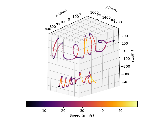
From the above plot, we can see that the speed is highest on long, straight strokes and lowest around kinks.

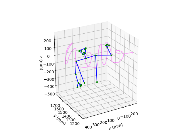
Visualise the skeleton

Next, we use the networkx package to define a graph based on a subset of keypoints. This allows us to more easily plot a skeleton of the upper-half of the individual.

# Select some keypoints from the "body" model
selected_body_kpts = [
    "body_nose",
    "body_left_eye",
    "body_right_eye",
    "body_left_shoulder",
    "body_right_shoulder",
    "body_left_hip",
    "body_right_hip",
    "body_left_elbow",
    "body_right_elbow",
    "body_left_wrist",
    "body_right_wrist",
    "body_left_index",
    "body_right_index",
    "body_left_pinky",
    "body_right_pinky",
    "body_left_thumb",
    "body_right_thumb",
    "body_left_ear",
    "body_right_ear",
    "body_mouth_left",
    "body_mouth_right",
]

# Select a frame index to extract the positions of the keypoints
body_frame = 130

# Initialize a graph
G = nx.Graph()

# Add nodes to the graph.
for kpt in selected_body_kpts:
    G.add_node(
        kpt,
        position=ds_hello.position.sel(time=body_frame, keypoints=kpt).values,
    )

# Add midpoint between the shoulders as node
G.add_node(
    "body_shoulders_midpoint",
    position=ds_hello.position.sel(
        time=body_frame,
        keypoints=["body_left_shoulder", "body_right_shoulder"],
    )
    .mean(dim="keypoints")
    .values,
)

# Add edges to the graph.
G.add_edge("body_right_shoulder", "body_left_shoulder")
for side_str in ["left", "right"]:
    G.add_edge(f"body_{side_str}_shoulder", f"body_{side_str}_elbow")
    G.add_edge(f"body_{side_str}_shoulder", f"body_{side_str}_hip")
    G.add_edge(f"body_{side_str}_elbow", f"body_{side_str}_wrist")
    G.add_edge(f"body_{side_str}_wrist", f"body_{side_str}_index")
    G.add_edge(f"body_{side_str}_wrist", f"body_{side_str}_pinky")
    G.add_edge(f"body_{side_str}_wrist", f"body_{side_str}_thumb")
    G.add_edge(f"body_mouth_{side_str}", f"body_{side_str}_ear")

# Add edge between the shoulders midpoint and the nose
G.add_edge("body_shoulders_midpoint", "body_nose")

# Add edge between the ears
G.add_edge("body_left_ear", "body_right_ear")

# Add edge across the mouth
G.add_edge("body_mouth_left", "body_mouth_right")

We can now use the above graph to plot the skeleton.

fig = plt.figure()
ax = fig.add_subplot(111, projection="3d")

# Get dictionary of node positions
# (key: node, value: (x, y, z))
positions_dict = nx.get_node_attributes(G, "position")

# Plot nodes of skeleton in green
for _node, (x, y, z) in positions_dict.items():
    ax.scatter(x, y, z, s=10, color="green")

# Plot edges of skeleton in blue
for edge in G.edges():
    node_1, node_2 = edge
    x1, y1, z1 = positions_dict[node_1]
    x2, y2, z2 = positions_dict[node_2]
    ax.plot([x1, x2], [y1, y2], [z1, z2], "b-")

# Plot the right index finger keypoint for the selected time window
# in magenta
ax.plot(
    right_index_position_hello.sel(space="x"),
    right_index_position_hello.sel(space="y"),
    right_index_position_hello.sel(space="z"),
    alpha=0.35,
    color="magenta",
)

ax.view_init(elev=25, azim=-120, roll=0)
ax.set_aspect("equal")
ax.set_xlabel("x (mm)")
ax.set_ylabel("y (mm)")
ax.set_zlabel("z (mm)")

# Invert x-axis to make traced text readable
ax.invert_xaxis()